Last week, I shared two different datasets on the views my website observed for this past week and future weeks:

1. A model’s prediction:

• Next 7 Days (08/02/2026): 91
• Current Calendar Month (01/02/2026 – 28/02/2026): 412
• Next Calendar Month (01/03/2026 – 31/03/2026): 483
• Next 3 Calendar Months (01/02/2026 – 30/04/2026): 1,376
• By 30th June (01/01/2026 – 30/06/2026): 2,896
• Last Half of Year (01/07/2026 – 31/12/2026): 3,353
• Full Year (31/12/2026): 6,249

2. My gut instinct:

• Next 7 Days (08/02/2026): 105
• Current Calendar Month (01/02/2026 – 28/02/2026): 450
• Next Calendar Month (01/03/2026 – 31/03/2026): 400
• Next 3 Calendar Months (01/02/2026 – 30/04/2026): 1,272
• By 30th June (01/01/2026 – 30/06/2026): 1,055
• Last Half of Year (01/07/2026 – 31/12/2026): 2,800
• Full Year (31/12/2026): 3,855

The total views that I had over this past week (02/02/2026 – 08/02/2026) was:

225

Updated Numbers

Turns out that neither the model nor my gut was accurate. Over the past 2 weeks, I’ve experienced 2 days of anomalies (outliers; +/-3 standard deviations from the mean). These were specifically: 27th January (147 views) and 6th February (99 views). An interesting difference between the two days is the 27th January saw 146 visitors, whereas 6th February saw 61 visitors. The average for both weeks were 37.13 and 32.14 respectively. All of this leads me to the question: which model was more reliable?

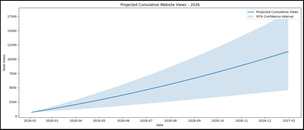
To test and put my own bias in check, I re-ran the model using the previous data, but this time including the anomalies, and this was output. This is really about putting this here as future evidence for December. Now, to think of a search term so that I can remember that it’s here; predicted 2026’s website forecasted views with anomalies/anomaly included. What I believe these numbers highlight is that SARIMAX can work well in the short-term regarding outliers, but will ultimately suffer from biasing the model upwards due to the change in variance:

• Next 7 Days (08/02/2026): 270
• Current Calendar Month (01/02/2026 – 28/02/2026): 618
• Next Calendar Month (01/03/2026 – 31/03/2026): 595
• Next 3 Calendar Months (01/02/2026 – 30/04/2026): 2,148
• By 30th June (01/01/2026 – 30/06/2026): 4,586
• Last Half of Year (01/07/2026 – 31/12/2026): 6,750
• Full Year (31/12/2026): 11,336

Differences

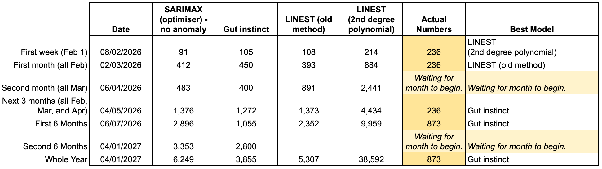
I’ve produced a table to make decision-making easier for myself. This table shows the Python output from 02/02/2026, my gut instinct, parts of the 2025 forecasting system (LINEST 1 and MULTEST (2 degree polynomials)), and the observed views across 2026. These are then broken down into specified date buckets. If you’ve read this post, you’ll know what I mean by MULTEST.

Reframing Thinking

Needless to say, I was thrilled to see more views than expected. Counter to this, part of me was annoyed that this didn’t land within the model’s projected output. Observing the past weekly median values between 2024 (6), 2025(9) (51), and 2026 (115), the data show the website is experiencing an increase in stable daily traffic. But, how do we handle these spikes?

In last week’s post was a note about averaging the days around these spikes to assist smoothing the data over. But the conclusion about these spikes is that they’re not noise, they are behaviour. Even though an average can be set for these days, it doesn’t truly reflect this fact in the model. When the anomalies are included in the model, the system blows out and my intuition tells me that these numbers are too big:

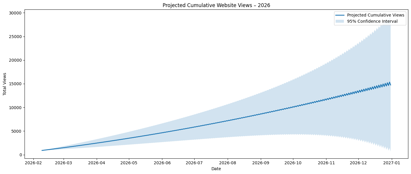
• Next 7 Days (ending 15/02/2026): 170
• Current Calendar Month (01/02/2026 – 28/02/2026): 813
• Next Calendar Month (01/03/2026 – 31/03/2026): 577
• Next 3 Calendar Months (01/02/2026 – 30/04/2026): 2,586
• By 30th June (01/01/2026 – 30/06/2026): 5,780
• Last Half of Year (01/07/2026 – 31/12/2026): 8,961
• Full Year (01/01/2026 – 31/12/2026): 14,741

Whilst hanging out the washing on the weekend, during some beautiful last moments of Tasmanian summer, the process was running through my head. Well, I’m assuming that it was one of the last hot summer days; I can’t predict the weather. Thinking about how spikes can blow forecasted values out, I thought of a few tactics that I could implement to help drive a bit more stable direction. Overall, the data is seeing growth change over time and the models that I am advised by aren’t taking that into account. The following are areas that I am going to delve into to see which main drivers are going to best suit the situation. My end goal is to maintain a clean and clear script that doesn’t overinflate the model; a drive for parsimony.

Next steps

1. Log transform views

The variance is increasing over time so I need to stabilise this by log transforming the data. In turn, this will also reduce the influence that outliers have on the forecast and improve their confidence intervals.

2. Add spike dummy variables

Whilst considering why a website might observe spikes in its data, e.g. Google influence, LinkedIn, job applications, etc, I realised that this model isn’t accounting for those influences. Instead of adding an average smoothing method, I’m thinking of implementing a median absolute deviation process to assist the model.

3. Add structural growth dummy variable

As I mentioned earlier, the year-on-year base views are growing over time; this makes sense given the impact that connecting to Google has made. By integrating this variable into the model, the ARIMA process won’t absorb the autoregressive term into its growth; more predictable forecasts (ceteris paribus).

4. Include day-of-week seasonality

Last week, I mentioned the negation of hourly data based on the trade-off of manually obtaining data and its potential benefits. As such, I believe that I can start to account for the day-of-the-week seasonality into the model. Even though I took a long break from creating content, I developed posts on LinkedIn in an attempt to maintain engagement. Due to these posts, it definitely did drive traffic and, at the very least, created awareness. Ultimately, I can search back through the data and find the mode days that the site observes the most traffic; yearly, quarterly, seasonally, etc.

5. Fit SARIMAX with exogenous regressors

Pool all of the exogenous regressors together and fit the model to those regressors. It makes sense to attempt an analysis based on this premise, especially as there is unknown (to my perspective) traffic to the website. Instead of categorising this as ‘organic traffic’, I’d prefer to search for the root cause. This exogenous regressor approach can provide some insights into this.

6. Validate on rolling windows

Maintain the rolling data validation, but actually sit with the data & analysis and critique the impacts and effects of the changes over time. If something doesn’t work, analyse it again using different parameters and attempt to make sense of why. If it’s not, wait another few months whilst attempting other approaches on the side. Why would I pull the car over every 5 minutes to question the route my GPS has chosen because the ETA time hasn’t decreased? Apparently, there’s a growing theme with me and travel time.

7. Change model to underlying GARCH approach

What 1-6 might also indicate is my brain digging in too far to a problem to solve it, rather than pulling up to another level and thinking, “what’s the problem that I’m trying to solve? Is this the right method to do so? What’s another angle I could take?” The Generalised Autoregressive Conditional Heteroskedasticity approach takes into consideration the volatility and constant change of variance in the data. What we’re interested in this model is the alpha attached to the residuals (epsilon): σ²_t = ω + α₁ε²_t-1 + β₁σ²_t-1. The ACF, PACF, and Ljung-Box Test output(s) are present to assist your analysis for the null hypothesis; standardised square errors are uncorrelated with history of levels, e.g. α₁ = α₁ = … = α_q = 0.

Let’s see what happens over the next week.