95 – How I Developed my Website Statistics Metrics

My Predictions

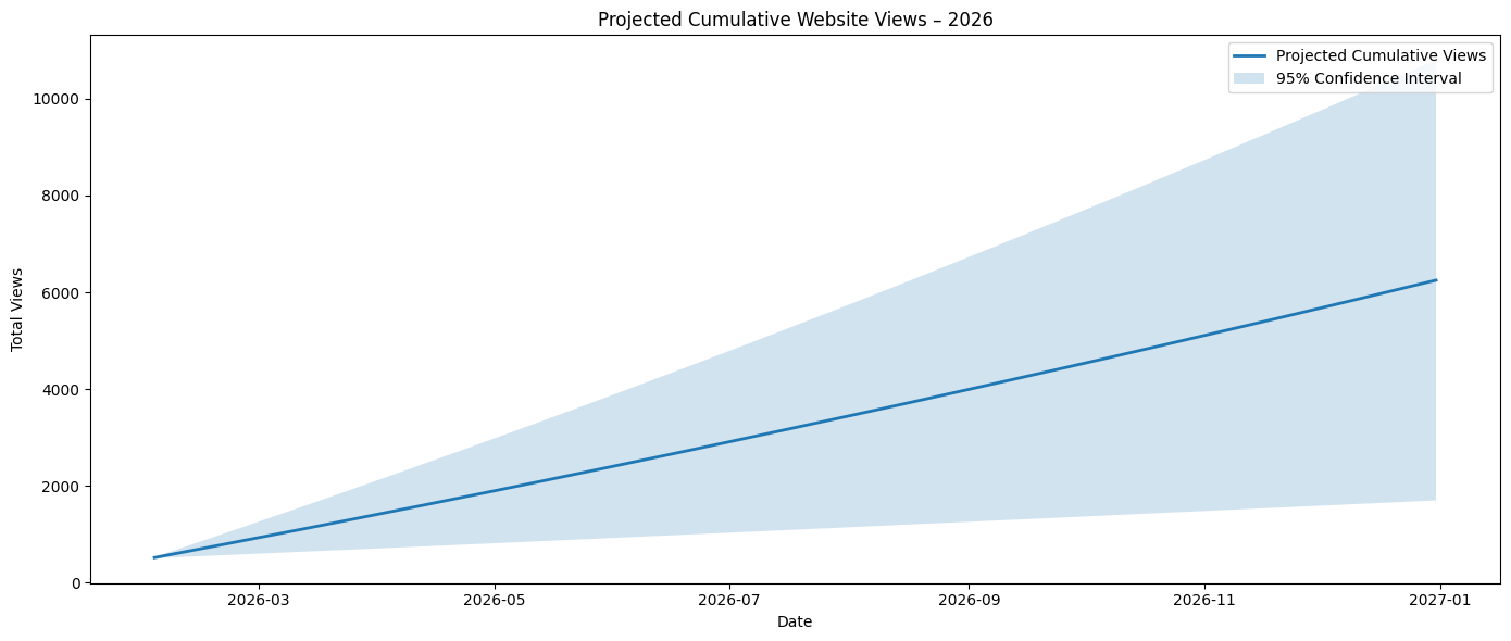
Below are my 2026 website statistics model’s* predictions for the:

Next 7 Days (08/02/2026): 91
Current Calendar Month (01/02/2026 – 28/02/2026): 412
Next Calendar Month (01/03/2026 – 31/03/2026): 483
Next 3 Calendar Months (02/05/2026): 1,376
By 30th June (01/01/2026 – 30/06/2026): 2,896
Last Half of Year (01/07/2026 – 31/12/2026): 3,353
Full Year (31/12/2026): 6,249

*I replaced an anomaly of 174 views on 27th January using the average method of the previous data point for the year; 15 views. The projected ‘Full Year’ forecast was 10,728; supposedly unlikely.

Below are my gut instinct 2026 website statistics predictions for the:

Next 7 Days (08/02/2026): 105
Current Calendar Month (01/02/2026 – 28/02/2026): 450
Next Calendar Month (01/03/2026 – 31/03/2026): 400
Next 3 Calendar Months (02/05/2026): 1,272
By 30th June (01/01/2026 – 30/06/2026): 1,055
Last Half of Year (01/07/2026 – 31/12/2026): 2,800
Full Year (31/12/2026): 3,855

Initial Model

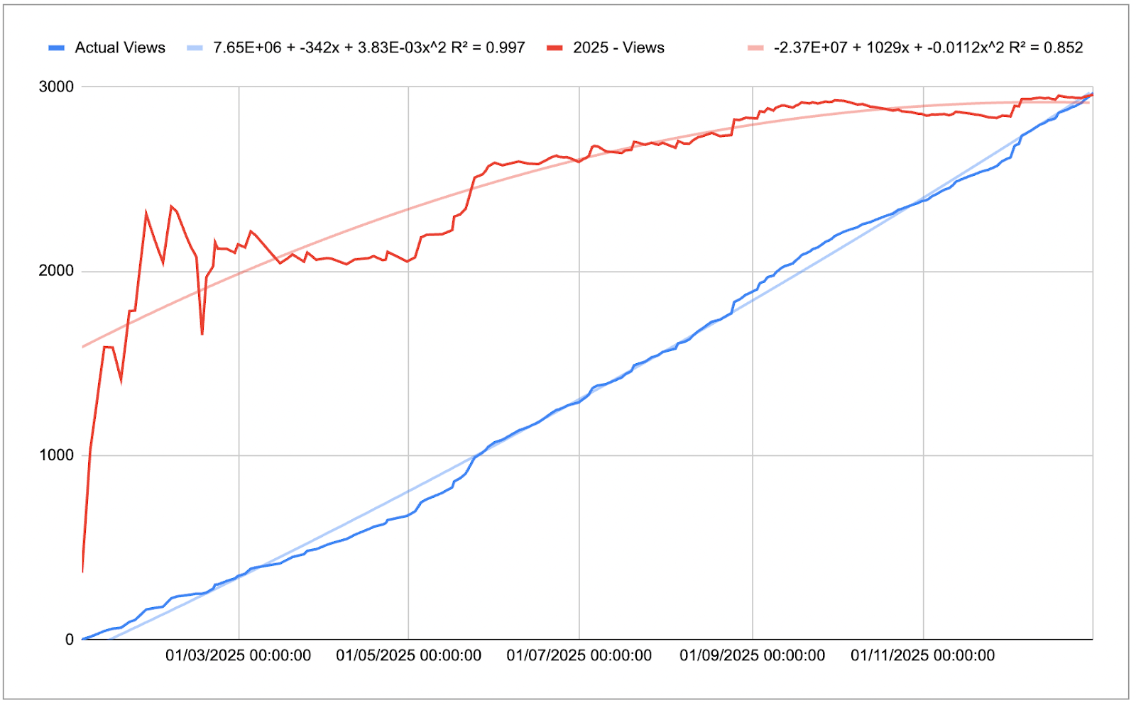
At the beginning of last month, this blog post was a summary of my 2025 website statistics where the data show change over time due to exogenous impacts on the system. Within that summary was the forecasted total number of views I expected the site to receive. That forecast, although reflecting a trend over time, was not reliable given the volatility of fluctuations in views per day. See Appendix A for details for how I calculated this over the year:

The process and model of how I developed this forecast is located in Appendix B for those wanting a deeper look into the data. Otherwise, you can also see in that previous post how the data is organised. This is not best practice as the analysis wasn’t truly separated from the dataset:

Essentially, I was looking for a way to forecast the final view count and track the history of projections. What you’re seeing is a self-constructed sunk cost fallacy system; add this bias back to the list. I fell into this fallacy through the fact that I had spent time setting it up and it….worked. Why fix it if it ain’t broke? Creating this flow became easy for me to use throughout the year as I only had to enter a few pieces of data, albeit manually. Still attempting to figure out how to stream this WordPress data; hopefully this is a positive foreshadowing thought.

This poor convolution of data storage and processing made for tedious data analysis. The main issue was that I didn’t have strict daily numbers, but an average over ‘x’ hours, e.g. 34 views over 71.7 hours. It should be necessary for me to explain the effect of outliers on the average, especially over a couple of days. Statology (Zach) has already done that work. I ended up pivoting and approached this question from a different angle.

Updated Process

Given the recent Python relearning and upskilling that I had commenced over the 2025/2026 work break through DataCamp, this presented me with a perfect opportunity to implement some of that new knowledge into a meaningful project. One of the pedagogical issues that I have with websites like DataCamp, Coursera, and Udemy is the fact that it’s a series of ‘complete this task then this one,’ rather than consolidating your learning in unit batches. There has been that transition towards ‘earn your certificate through our [affiliation link]’, but this batching isn’t ultimately integrated into the programs themselves.

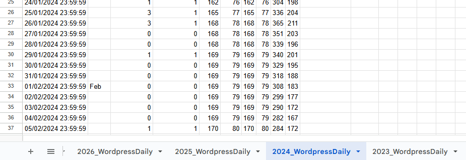
From the predictions at the beginning of this post, I was interested in various types of analysis to see if there was a particular point where the predictor gets too far off. To achieve this, I wanted more granular data so I decided to accumulate my website’s daily views and visitors from 2023 onwards. Although I can see the potential benefit for retrieving the time data, the payoff for the current manual method didn’t seem worth it. I placed each separate year into its own tab then collated them:

I used the collection of VSTACK, QUERY, and SORT to arrange all of the data:

=SORT(QUERY(VSTACK(‘2026_WordpressDaily’!A2:D,’2025_WordpressDaily’!A2:D,’2024_WordpressDaily’!A2:D,’2023_WordpressDaily’!A2:D),”SELECT Col1, Col3, Col4″),1,1)

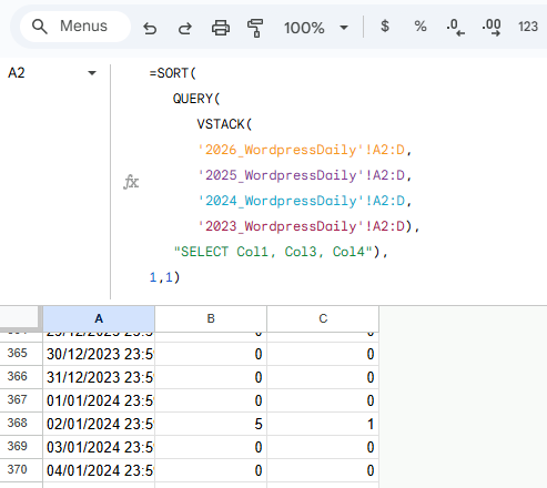
VSTACK was used to place each one on top of the other, QUERY was used to eliminate the second column (month differentiation signifier) that I was using for visual ease, and SORT was used for two reasons; move all blank cells to the bottom and reorganise any years that were out of order when placing the arrays in VSTACK.

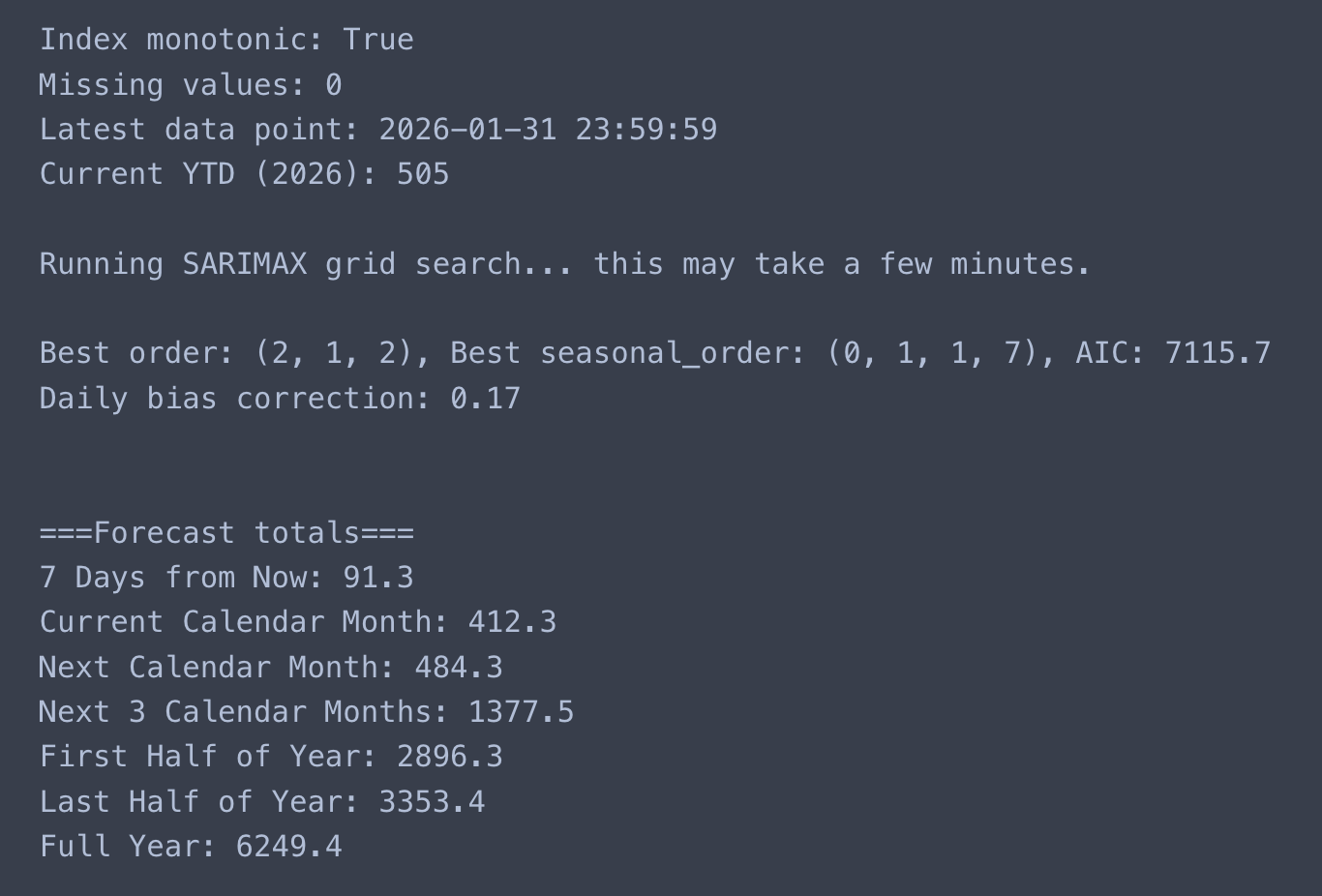
Gathering at this level allows for an increase in accurate analysis for seasonal change, depending on the content and SEO tags that have been assigned to the site’s web pages. I’ve included 2 Python scripts in Appendix D that highlight two different approaches. The first script forecasts the various time periods in 2026 using a fixed SARIMAX approach. Specifically, it assumes that the autoregressive, integration, and moving average parameters are 1. Similarly, the seasonal order has the same parameters, except for the seasonal period being 7 (days). This script is what I used for my final predictions.

The main learnings that I was able to implement in this project were:

The understanding and use of iloc over loc (5. Forecast helper function with bias correction),
Integration of dictionaries and outputs (7. Run forecasts and output), and
Iterative test storage and comparison of parameters in the SARIMAX function; isolating the ideal AIC, order, and seasonal order (2. Hyperparameter tuning (best order)).

Although my intent is to post a weekly blog from here, I can’t explain how much energy it took me to create this one. However, I do aim to release the periodic views to see how the model stacked up against reality. I’m genuinely looking forward to seeing how I can update the predictor based on factors that I can track.

I thought I would create a table for each of the next posts for this series, updating the entries in the table for each date and the different models used:

Date	SARIMAX (optimiser) – no anomaly	Gut instinct	LINEST (old method)	LINEST (2nd degree polynomial)
09/02/2026	91	105	108	214
02/03/2026	412	450	393	884
06/04/2026	483	400	891	2,441
04/05/2026	1,376	1,272	1,373	4,434
06/07/2026	2,896	1,055	2,352	9,959
04/01/2027	6,249	3,855	5,307	38,592

Appendices

Appendix A – Calculating the Year’s Total Views

Here is the formula developed to calculate/estimate the year’s total views:

=G4/((NOW()-DATE(YEAR(NOW()),1,1))/(DATE(YEAR(NOW()),12,31)-DATE(YEAR(NOW()),1,1)))

Where G4 is the total number of views at any given point in time.

We can put this into words by saying:

Current total views divided by percentage of the year that has passed.

The intuition behind this is that it projects the number of views forward by the percentage of the year that’s passed. If I had 1 view on 1st January, I’m interested to know how many views I could receive over the year. So, I would use the formula:

= Views / Percentage of the year that’s passed

= 1 / (1/365)

= 1 / 0.0027

= 365

If I have the following views data for the first 5 days of the year, I can make an estimate for the end of the year; 1, 5, 6, 3, 7:

= Views / Percentage of the year that’s passed

= (1+5+6+3+7) / (5/365)

= 22 / 0.0137

= 1,606

Assuming 360 days have passed and I’ve received 1,390 views:

= Views / Percentage of the year that’s passed

= 1,390 / (360/365)

= 1,390 / 0.9863

= 1,409

Appendix B – Approaching 2025’s Analysis

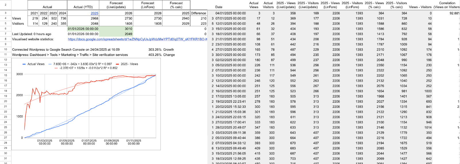
Unsure how each method would stack up against one another, I decided to run a test for each one alongside one another. To complete this they all required the previous years’ data; a simple copy-paste from WordPress.

Gathering the dataset

Actual (YTD) was the variable that I was manually updating periodically throughout the year. Here, I entered the cumulative views and visitors that had hit the website.

Actual					Actual (YTD)
Year	2021	2022	2023	2024	2025
Views	219	254	502	736	2891
Visitors	114	129	240	355	1985

This portion of the table was where each row was dependent on values being updated in the Actual (YTD) cells.

Forecast (LiveUpdate)		Forecast (LinFore)		Forecast (% calc)
2026		2026		2025
2668	=FORECAST.LINEAR(G$3,$B4:$F4,$B$3:$F$3)	2668	=FORECAST.LINEAR(H$3,$B$4:$F$4,$B$3:$F$3)	2936	=F4/((NOW()-DATE(2025,1,1))/(DATE(2025,12,31)-DATE(2025,1,1)))
1755	=FORECAST.LINEAR(G$3,$B5:$F5,$B$3:$F$3)	1755	=FORECAST.LINEAR(H$3,$B$5:$F$5,$B$3:$F$3)	2016	=F5/((NOW()-DATE(2025,1,1))/(DATE(2025,12,31)-DATE(2025,1,1)))

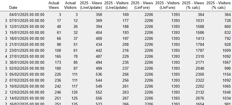
This following is a subset of the output that it produced:

Metrics

Testing the accuracy of the various analysis types led me to creating this table of metrics, showing predicted dates, that would update with new data being added to the sheet.

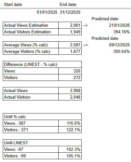
Actual Views Estimation

=INTERCEPT(M3:M,$L$3:$L)+SLOPE(M3:M,$L$3:$L)*$Y$3

M3:M: Actual Views
L3:L: Date
Y3: End date

Actual Visitors Estimation

=INTERCEPT(N3:N,$L$3:$L)+SLOPE(N3:N,$L$3:$L)*$Y$3

N3:N: Visitors
L3:L: Date
Y3: End date, e.g. 31/12/2025

Predicted date [to achieve the Actual Views Estimation]:

=LET(today,TODAY(),

beg,X3,

compFore,Y24,

beg+((today-beg)/compFore))

X3: Start date, e.g. 01/01/2025
Y24: Actual Views/Actual Views Estimation
- How close is the real-world data to the model’s forecast of the number of estimated views by the end date?
today-beg: number of days between today’s date and the beginning date of this model
(today-beg)/compFore): add the number of days remaining for the forecast to match the real-world data
beg+((today-beg)/compFore)): count the number of days from the beginning date of this model, e.g. the estimated date you will see the predicted number of views on the website.

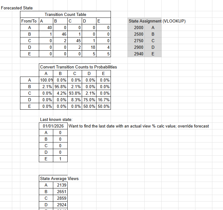
Appendix C – The Quandary for Markov Chains

This is what got my brain thinking about Markov Chain analysis for this project. I noticed that the forecasted views (red) closely resembled the distribution of ‘n’ number of coin flips:

Naturally, I started considering this law of large numbers. To make the best reference possible to this idea, here I’ve plotted a map of 100 coin flips and the average outcome:

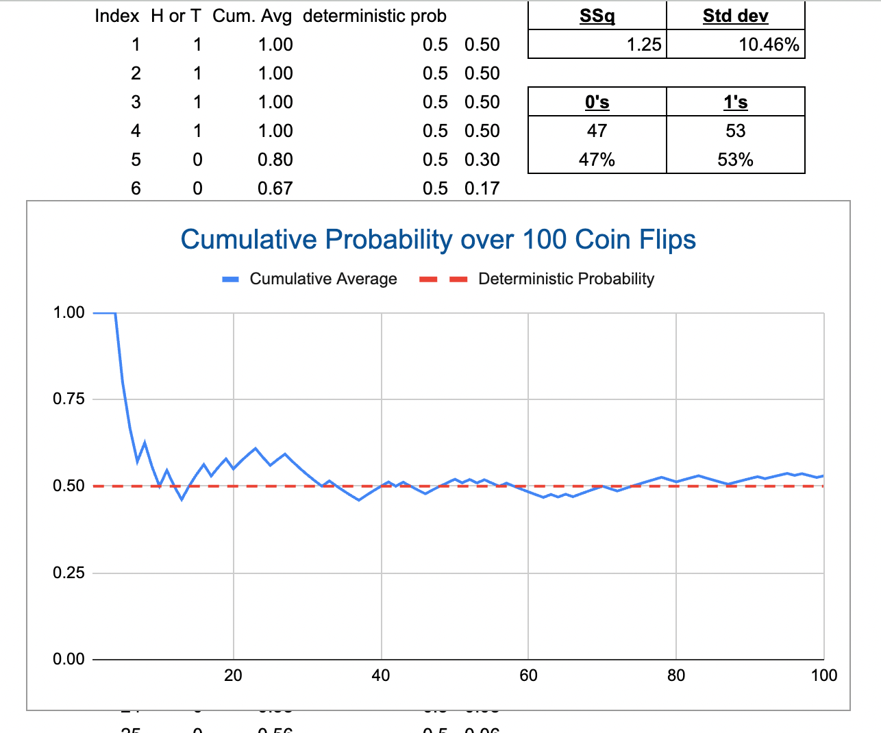
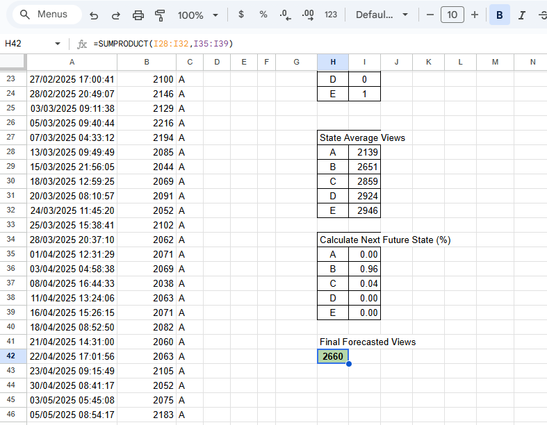
Although my Markov Chain analysis came to an impasse for this project, I decided to see what the best calculating I could predict; 2,660:

Appendix D – Python Scripts

Script 1

### Forecasting various time periods in 2026 ###

import pandas as pd

from statsmodels.tsa.statespace.sarimax import SARIMAX

# =========================

# 1. Load and prepare data

# =========================

URL = “https://docs.google.com/spreadsheets/d/12XxYn4zgcHVMJfme0rvQRA4eyJe9y005nc8Jx2DM9f8/export?format=csv&gid=1047244059”

# Read CSV and parse dates

df = pd.read_csv(URL, parse_dates=[“Date”], dayfirst=True)

# Sort and set index

df = df.sort_values(“Date”)

df = df.set_index(“Date”)

# Fill missing values with 0

df[“Actual Views”] = df[“Actual Views”].fillna(0)

# Force daily frequency

df = df.asfreq(“D”, fill_value=0)

# Check data integrity

print(“Index monotonic:”, df.index.is_monotonic_increasing)

print(“Missing values:”, df.isnull().sum().sum())

print(“Latest data point:”, df.index.max())

print(“Current YTD (2026):”, df.loc[df.index.year == 2026, “Actual Views”].sum())

# =========================

# 2. Fit SARIMAX model

# =========================

model = SARIMAX(

df[“Actual Views”],

order=(1,1,1),

seasonal_order=(1,1,1,7),

enforce_stationarity=False,

enforce_invertibility=False

)

results = model.fit(disp=False)

# =========================

# 3. Forecast helper function

# =========================

def forecast_period(start_date, end_date):

“””Forecast total views from start_date to end_date inclusive”””

last_observed = df.index.max()

# Number of days to forecast

forecast_days = (end_date – last_observed).days

forecast_days = max(forecast_days, 0)

# Actual observed in period

actual_period = df.loc[(df.index >= start_date) & (df.index <= end_date), “Actual Views”].sum()

# Forecast if days remain

if forecast_days > 0:

forecast = results.get_forecast(steps=forecast_days)

mean = forecast.predicted_mean

conf = forecast.conf_int()

total = actual_period + mean.sum()

lower = actual_period + conf.iloc[:, 0].sum()

upper = actual_period + conf.iloc[:, 1].sum()

else:

total = actual_period

lower = actual_period

upper = actual_period

return {“Actual”: actual_period, “Forecast”: total, “CI Lower”: lower, “CI Upper”: upper}

# =========================

# 4. Define forecast periods

# =========================

today = pd.Timestamp.now().normalize()

current_year = today.year

periods = {

“7 Days from Now”: (today, today + pd.Timedelta(days=6)),

“Current Calendar Month”: (pd.Timestamp(today.year, today.month, 1),

pd.Timestamp(today.year, today.month, 1) + pd.offsets.MonthEnd(0)),

“Next Calendar Month”: (pd.Timestamp(today.year, today.month, 1) + pd.offsets.MonthBegin(1),

pd.Timestamp(today.year, today.month, 1) + pd.offsets.MonthEnd(1)),

“Next 3 Calendar Months”: (pd.Timestamp(today.year, today.month, 1) + pd.offsets.MonthBegin(1),

pd.Timestamp(today.year, today.month, 1) + pd.offsets.MonthEnd(3)),

“First Half of Year”: (pd.Timestamp(current_year, 1, 1), pd.Timestamp(current_year, 6, 30)),

“Last Half of Year”: (pd.Timestamp(current_year, 7, 1), pd.Timestamp(current_year, 12, 31)),

“Full Year”: (pd.Timestamp(current_year, 1, 1), pd.Timestamp(current_year, 12, 31))

}

# =========================

# 5. Run forecasts and output

# =========================

results_dict = {}

for name, (start, end) in periods.items():

results_dict[name] = forecast_period(start, end)

# Print results nicely

for name, values in results_dict.items():

print(f”\n=== {name} ===”)

print(f”Actual Observed: {values[‘Actual’]}”)

print(f”Forecast Total: {values[‘Forecast’]:.1f}”)

print(f”95% CI Lower: {values[‘CI Lower’]:.1f}”)

print(f”95% CI Upper: {values[‘CI Upper’]:.1f}”)

# Print forecasts only

print(“\n\n===Forecast totals===”)

for name, values in results_dict.items():

print(f”{name}: {values[‘Forecast’]:.1f}”)

residuals = results.resid

residuals.plot(title=”Residuals”)

Script 2

### Forecasting various time periods in 2026 ### COMBINED WITH ### Auto-updating SARIMAX order and seasonal_order parameters ###

import pandas as pd

import itertools

import warnings

from statsmodels.tsa.statespace.sarimax import SARIMAX

import matplotlib.pyplot as plt

warnings.filterwarnings(“ignore”)

# =========================

# 1. Load and prepare data

# =========================

URL = “https://docs.google.com/spreadsheets/d/12XxYn4zgcHVMJfme0rvQRA4eyJe9y005nc8Jx2DM9f8/export?format=csv&gid=1047244059”

df = pd.read_csv(URL, parse_dates=[“Date”], dayfirst=True)

df = df.sort_values(“Date”).set_index(“Date”)

df[“Actual Views”] = df[“Actual Views”].fillna(0)

df = df.asfreq(“D”, fill_value=0)

df.index = pd.to_datetime(df.index)

print(“Index monotonic:”, df.index.is_monotonic_increasing)

print(“Missing values:”, df.isnull().sum().sum())

print(“Latest data point:”, df.index.max())

print(“Current YTD (2026):”, df.loc[df.index.year == 2026, “Actual Views”].sum())

# =========================

# 2. Hyperparameter tuning (best order)

# =========================

print(“\nRunning SARIMAX grid search… this may take a few minutes.”)

p = d = q = range(0, 3)

P = D = Q = range(0, 2)

s = 7 # weekly seasonality

pdq = list(itertools.product(p, d, q))

seasonal_pdq = list(itertools.product(P, D, Q))

best_aic = float(“inf”)

best_order = None

best_seasonal_order = None

for order_candidate in pdq:

for seasonal_candidate in seasonal_pdq:

try:

model = SARIMAX(

df[“Actual Views”],

order=order_candidate,

seasonal_order=(seasonal_candidate[0], seasonal_candidate[1], seasonal_candidate[2], s),

enforce_stationarity=False,

enforce_invertibility=False

)

results_test = model.fit(disp=False)

if results_test.aic < best_aic:

best_aic = results_test.aic

best_order = order_candidate

best_seasonal_order = (seasonal_candidate[0], seasonal_candidate[1], seasonal_candidate[2], s)

except:

continue

print(f”\nBest order: {best_order}, Best seasonal_order: {best_seasonal_order}, AIC: {best_aic:.1f}”)

# =========================

# 3. Fit SARIMAX with best params

# =========================

model = SARIMAX(

df[“Actual Views”],

order=best_order,

seasonal_order=best_seasonal_order,

enforce_stationarity=False,

enforce_invertibility=False

)

results = model.fit(disp=False)

# =========================

# 4. Compute bias from residuals

# =========================

residuals = results.resid

bias_daily = residuals.mean()

print(f”Daily bias correction: {bias_daily:.2f}”)

# =========================

# 5. Forecast helper function with bias correction

# =========================

def forecast_period(start_date, end_date):

“””Forecast total views from start_date to end_date inclusive with bias correction”””

last_observed = df.index.max()

forecast_days = (end_date – last_observed).days

forecast_days = max(forecast_days, 0)

actual_period = df.loc[(df.index >= start_date) & (df.index <= end_date), “Actual Views”].sum()

if forecast_days > 0:

forecast = results.get_forecast(steps=forecast_days)

mean = forecast.predicted_mean – bias_daily # apply daily bias correction

conf = forecast.conf_int()

conf_lower = conf.iloc[:, 0] – bias_daily

conf_upper = conf.iloc[:, 1] – bias_daily

total = actual_period + mean.sum()

lower = actual_period + conf_lower.sum()

upper = actual_period + conf_upper.sum()

else:

total = actual_period

lower = actual_period

upper = actual_period

return {“Actual”: actual_period, “Forecast”: total, “CI Lower”: lower, “CI Upper”: upper}

# =========================

# 6. Define forecast periods