In one of my current jobs, it’s my responsibility to track updates in timetables. For any event that we plan for, it’s necessary to have between 6 and 20 workers assigned on a day. However, given the nature of work, life, and competing priorities, some people will need to bow out from these events, leaving space for others to step in on their behalf. The thing is, I’m not the point-person who gets alerts of these changes in the workers’ priorities. All I see is a spreadsheet with names highlighted, indicating that they have been swapped.

I operate on two different sources; a master spreadsheet that maintains the master (up-to-date and accurate) data of assigned workers, and an auxiliary sheet, where I update the changes that have been made. Subsequently, I change settings in other software within the pipeline for future automated operations. The order of names on the Master spreadsheet is stagnant (with only names being replaced by those who bow out) and the order of names on the Auxiliary spreadsheet can be reordered over time, especially as varying people bow out.

Being cognisant of how much time was being spent on accurately identifying colleague swaps, I wanted to develop a tool that had the ability to cut this meticulous task time down. This tool that I have created has actually reduced my work time by 50% (what would have taken me 30 minutes now only takes me 15 minutes).

For this tool that I have created, and what you could hopefully utilise, it comes with some key assumptions that you would need to consider before implementing this solution into your workflow. To be honest with you, I love the fact that there are some “roadblocks” or constraints here as it means I now have the joy of finding solutions to cut this assumptions list down.

Assumptions

1. There are two key files being tracked; one master and one auxiliary:
   1. The master is the files where the first changes are being made,
   2. The auxiliary is the file that is changed after you have been notified about the changes in the master file,
2. Names (text) in both resources are the same,
3. No two names are unique,
   1. If so, would suggest using an ID approach to this problem,
4. Exact swaps are not accurate:
   1. If you’re meaning to swap John for Jane, and Jack for Julie, it might actually show as swapping John for Julie and Jane for Jack,
   2. At the end of the day, the people who are meant to be out are out and those who are meant to be in are in, and
5. The list lengths are of equal value.

https://docs.google.com/spreadsheets/d/1Qo-YmTdt4BkQvSi9UAOnjKWYznHpSygg5b8itmxz0hQ/edit?gid=0#gid=0

Process

What I’m outlining here is a mixture of approaches. It includes the process of how names can appear in the list and how I set out to solve the problem.

Enter Names

First, I obtained a list of names from an internet source for some unknown reason (see FAQ #10):

Michael Scott

Dwight Schrute

Jim Halpert

Pam Beesly

Ryan Howard

Andy Bernard

Robert California

Stanley Hudson

Kevin Malone

Meredith Palmer

Angela Martin

Oscar Martinez

Phyllis Vance/Lapin

Roy Anderson

Jan Levinson

Next, I duplicated the list the list of names:

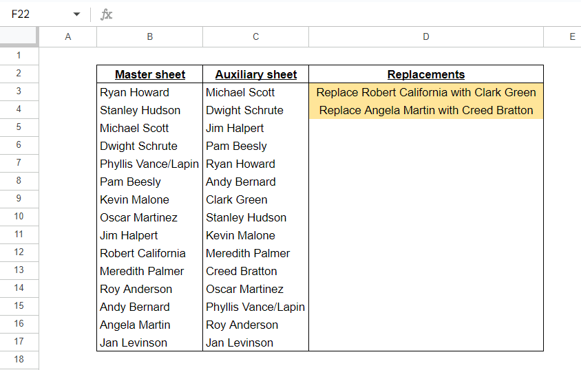
Then, I replaced two names in list found in the first column:

• Robert California with Clark Green, and
• Angela Martin with Creed Bratton

Shuffle the names in the first list:

Master sheet

I’m interested in finding how many matched names are in both of the lists and I can find this by using the MATCH function. Using the A column as the search key and the B column as the range, the following function will output the item number where a match exists. It will also report back no matches by showing an error:

=MATCH($A$2:$A,$B$2:$B, 0)

I can now convert these values into TRUE and FALSE by wrapping this formula in a ISNA function:

=ARRAYFORMULA(ISNA(MATCH($A$2:$A,$B$2:$B, 0)))

To retrieve the names of the people who match the TRUE values, I can wrap this formula in the FILTER function, and reference the A column, since these are the names that I am currently searching for:

=FILTER($A$2:$A,(ISNA(MATCH($A$2:$A,$B$2:$B, 0)))

Auxiliary Sheet

I can now follow the same process for the Auxiliary sheet:

=FILTER($B$2:$B,(ISNA(MATCH($B$2:$B,$A$2:$A, 0)))

Replacements

The main thing that we’re trying to achieve in this replacements section is find the names located in the Master sheet that are not in the Auxiliary sheet. Since we’re going to work with the FILTER function, it means that we no longer need to navigate the ARRAYFORMULA function as FILTER is going to deal with these arrays. First, I’ll start by concatenating the filters in columns C and D together in Column C. I want to be told who is to be replaced by whom. The master sheet holds the updated information, so I will want it to tell me who, in the master sheet, has been replaced:

=“Replace “ & 

FILTER($A$2:$A,(ISNA(MATCH($A$2:$A,$B$2:$B, 0))) & 

” with “ & 

FILTER($B$2:$B,(ISNA(MATCH($B$2:$B,$A$2:$A, 0)))

We can see that this has worked (for the first entry), but we need to apply it to the entire list and account for 2 types of criteria — the length of the list in columns A and B.

• If there are characters to be counted in column A, then I want it to be included, and
• If there are characters to be counted in column B, then I want it to be included.

We can achieve this by applying the same FILTER function for columns A and B into the conditional arguments for the FILTER function. However, we’ll wrap them in a LEN() function and check whether there exists strictly more than 0 characters in the cell(s).

=FILTER(“Replace “ & 

FILTER($A$2:$A,(ISNA(MATCH($A$2:$A,$B$2:$B, 0))) & 

” with “ & 

FILTER($B$2:$B,(ISNA(MATCH($B$2:$B,$A$2:$A, 0))),

LEN(FILTER($A$2:$A,(ISNA(MATCH($A$2:$A,$B$2:$B, 0)))) > 0,

LEN(FILTER($B$2:$B,(ISNA(MATCH($B$2:$B,$A$2:$A, 0)))) > 0,

Cleaner Code

Given what I’ve said in this previous post about updating my mindset, I want to make sure that this is as user-friendly as possible. So, I’ll make sure that I clean the code up by removing the cumbersome repetitive code and substitute it with the LET function:

=LET(Master, FILTER($A$2:$A,(ISNA(MATCH($A$2:$A,$B$2:$B, 0))),

Auxiliary, FILTER($B$2:$B,(ISNA(MATCH($B$2:$B,$A$2:$A, 0))),

FILTER(“Replace “ & Master & ” with “ & Auxiliary, 

LEN(Master) > 0, 

LEN(Auxiliary) > 0))

If you compare the two formulas side-by-side, I would posit that this LET perspective is much easier to read; variable name 1, variable function, variable name 2, variable function 2, formula with variable names.

Formatting

The last bits that I need to do is format the sheet a bit better, including a column name, conditional formatting (to search for the text ‘Replace’) in column C, and formatting of the column itself:

Conclusion

Hopefully, you have found this post and have also found it helpful for your situation. If you’ve used this solution, or adapted it in any way, I would love to see your results. Please comment below how you’ve utilised it.