
If you’ve been following this series, you would have seen my initial post (Part I) and subsequent post (Part II). If you’re not up to speed, I’m attempting to forecast my website views over time. I’ve started with a fairly simple model and I’m adjusting it over time to see how accurate I can make it. Here is how it’s been tracking so far:
| Timeframe | Part I (F) | Actual (to calendar date) | Part II (F) | Actual (to calendar date) | Wk 3 (F) | Actual (to calendar date) |
| 2nd Feb – 8th Feb; 9th Feb – 15th Feb; 16th Feb – 22nd Feb | 91 | 225 | 170 | 136 | 145 | 146 |
| February | 412 | 57 | 813 | 257 | 676 | 530 |
| March | 483 | 577 | 292 | |||
| February – April | 1,376 | 57 | 2,586 | 257 | 1,909 | 530 |
| January – June | 2,896 | 649 | 5,780 | 894 | 4,788 | 1,298 |
| July – December | 3,353 | 8,961 | 7,101 | |||
| January – December | 6,249 | 649 | 14,741 | 894 | 11,889 | 1,167 |
Of course the week where I don’t post the next week’s forecast is the one where the week’s (16th Feb – 22nd Feb) prediction is off by one view. You just got to trust me on this one.
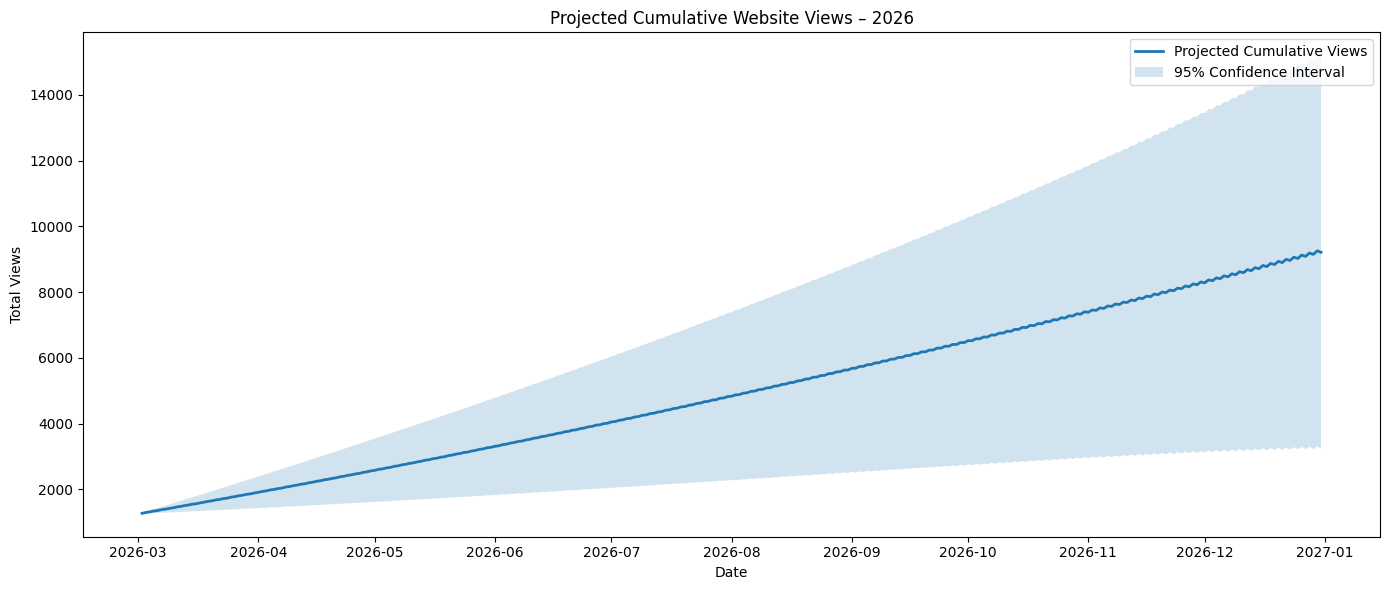
Below are the next forecasted views:
- Next 7 Days (01/03/2026 – 08/03/2026): 124
- Current Calendar Month (01/03/2026 – 31/03/2026): 633
- Next Calendar Month (01/04/2026 – 30/04/2026): 633
- Next 3 Calendar Months (01/03/2026 – 31/05/2026): 2,020
- First Half of Year (01/01/2026 – 30/06/2026): 4,014
- Last Half of Year (01/07/2026 – 31/12/2026): 5,198
- Full Year (31/12/2026): 9,212
Thoughts
I think what’s important is to track the changes being made. Common practice is to continuously evolve without appropriate reflection on where you started and the changes made. These posts outline maintaining multiple models and tracking the efficiency of each one, highlighting both good and bad decisions.
Although this isn’t a continuous integration/continuous development (CI/CD) system, I’ve been thinking of this DevOps methodology when applying it to this context. Yes, my “production” is just me, but it is a code that I run weekly to gather insights. In my rant post last week, I made reference to DORA. I’ll be pulling that back in this week, but specifically the 4 DORA metrics for measuring two critical aspects of DevOps (I’ve crossed out the metrics that don’t actually pertain to this use case):
- Velocity metrics track how quickly your organisation delivers software:
- Deployment frequency: How often code is deployed to production,
Lead time for changes: How long it takes code to reach production,
- Stability metrics measure your software’s reliability:
Change failure rate: How often deployments cause production failures,Time to restore service: How quickly service recovers after failures.
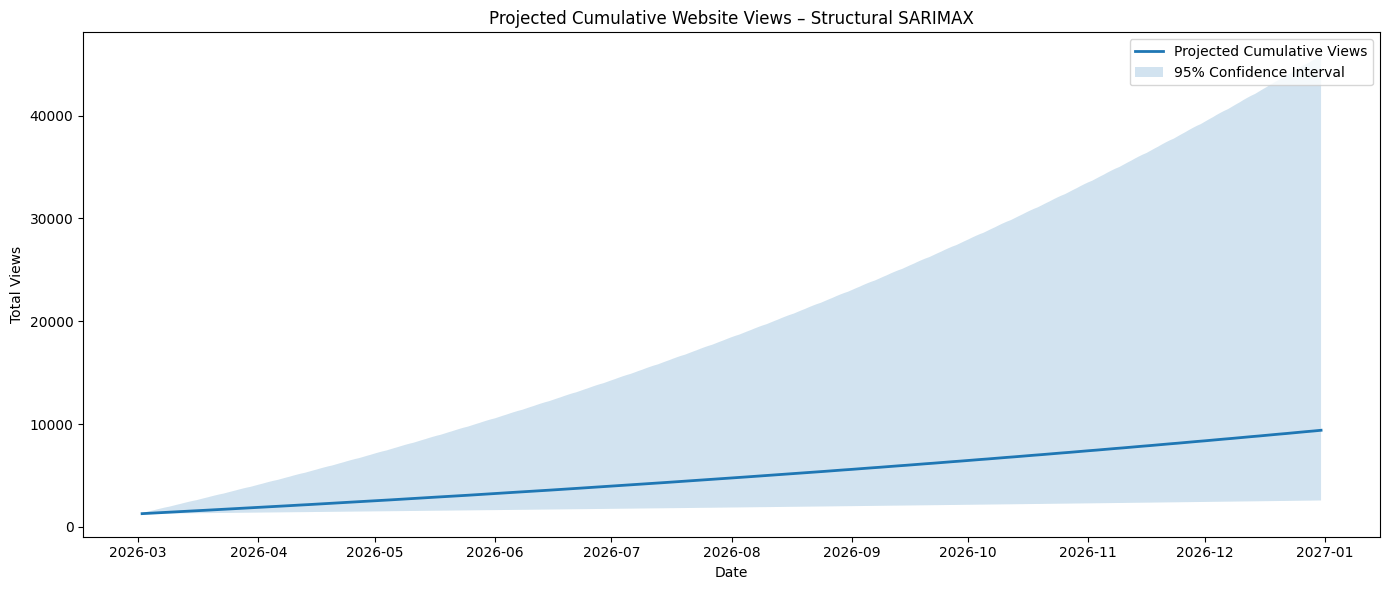
If this were a larger business, I would be discussing the efficacy of the models regarding their input/outputs and where we can make trade-offs for forecasting ability. In the Part II post, there’s an outline of these suggested trade-offs/next steps indicating various avenues to take the model. The results are developing an elongated decision tree with tracked code for each branch that you’ve created (welcome to Git):
Latest Code Update
Whilst considering the forecasted numbers above, in combination with their confidence intervals (CIs), I realised that I was attempting to make the model fit the data as opposed to help drive the model’s accurate and consistent (where possible) output. Ultimately, this is an incremental approach to updating model(s) where I’ll be analysing the efficacy and accuracy over several months. This approach has come from years of experience from creating too many projects in data, music, written assignments, etc., where the considered number of branches has not been correctly documented. This has often resulted in inaccurate reflection. Resolution can also signal the potential end for a model/analysis methodology.
I’ve spent time considering how to approach this forecasting problem, especially using the next steps from that previous post (Part II). As a reminder, here are the options that I considered:
- Log transform views
- Add spike dummy variables
- Add structural growth dummy variable
- Include day-of-week seasonality
- Fit SARIMAX with exogenous regressors
- Validate on rolling windows
- Change model to underlying GARCH approach
I reordered the list based on the script that I was using at the time, keeping the Log transformation option at the top, mainly due to it being an easy lift:
- Log transform views
- Fit SARIMAX with exogenous regressors
- Add spike dummy variables
- Add structural growth dummy variable
- Include day-of-week seasonality
- Validate on rolling windows
- Change model to underlying GARCH approach
Spoiler alert: Whilst integrating these different approaches, I was noticing that the confidence intervals were growing and the forecasted values were moving a fair bit.
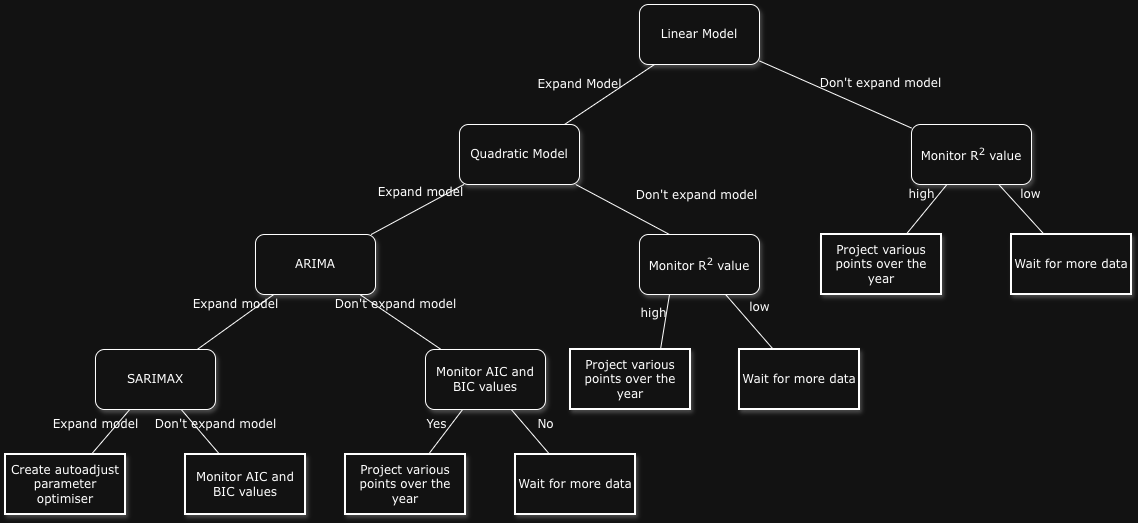
The Log Transformation Views process has been selected because it sets to stabilise the variance, account for seasonality, and convert the form of observed growth into a linear trend. Below are the output values I was receiving:
===Forecast totals===
01/03/2026 – 07/03/2026: 106
01/03/2026 – 31/03/2026: 527
01/04/2026 – 30/04/2026: 527
01/03/2026 – 31/05/2026: 1,610
01/01/2026 – 30/06/2026: 3,406
01/07/2026 – 31/12/2026: 3,275
01/01/2026 – 31/12/2026: 6,681
As you can imagine, I was satisfied with this output. My intuition says that the expected final outcome is lower than I would expect; we’re 1/6 of the way through the year and already at 1,262. I think about it in two ways, ceteris paribus:
- Monthly percentage of the year, and
1,262/(1/6) = 7,572
- Solve for x by cross multiplication, where x = total year views and views = time;
1,262 views in 31+28 days,
1,262 = 59 days
x views = 365 days
1,262*365 = 59x
x = 1,262*365/59
x = 7,807
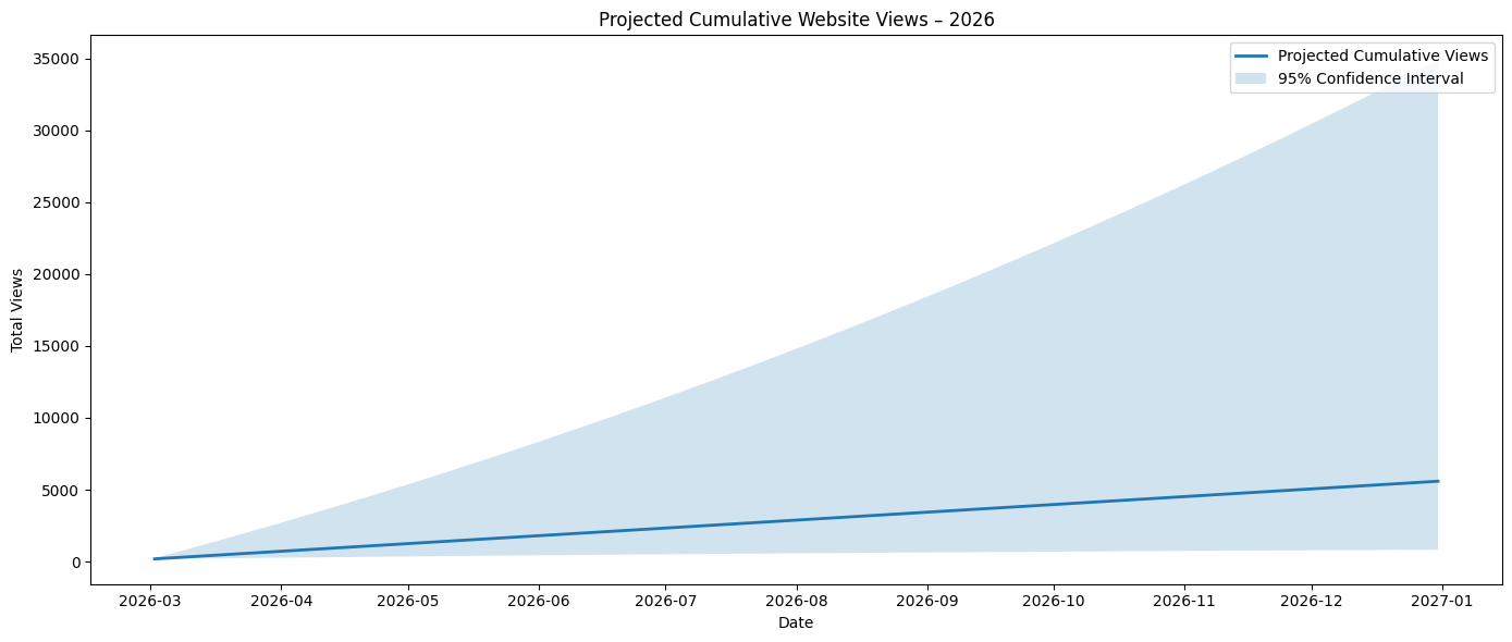
I continued on this journey of lower confidence intervals, whilst maintaining a realistic end output given how the data is trending. Next was Fit SARIMAX with exogenous regressors. Since SARIMAX already supports exogenous variables, I combined my Google Search Console data and ran the analysis. I chose to do this in an attempt to observe any potential spurious correlations and how to derive that third, fourth, or ninth causal factor. Due to the timeliness of the Google data availability, there is a 3 day lag and it doesn’t provide the most accurate and timely reference points:
===Forecast totals===
01/03/2026 – 07/03/2026: 121
01/03/2026 – 31/03/2026: 605
01/04/2026 – 30/04/2026: 605
01/03/2026 – 31/05/2026: 1,324
01/01/2026 – 30/06/2026: 3,932
01/07/2026 – 31/12/2026: 5,433
01/01/2026 – 31/12/2026: 9,392
I also attempted a few different libraries on the data that I integrated, specifically prophet and xgboost. I’m going to run them in parallel over the next month to critique their validity, but I observed that, for my use case and current dataset, the confidence intervals (CIs) and forecasted views for prophet were wider and tracking alongside the original model(s), whereas the same aspects for xgboost were narrower CIs but lower (unlikely) view counts for the different time periods.
Prophet
===Forecast totals===
01/03/2026 – 07/03/2026: 86
01/03/2026 – 31/03/2026: 615
01/04/2026 – 30/04/2026: 615
01/03/2026 – 31/05/2026: 811
01/01/2026 – 30/06/2026: 2,912
01/07/2026 – 31/12/2026: 2,506
01/01/2026 – 31/12/2026: 5,431
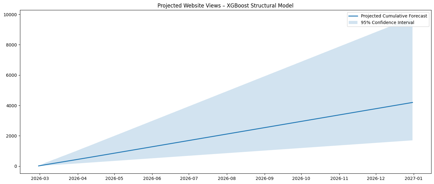
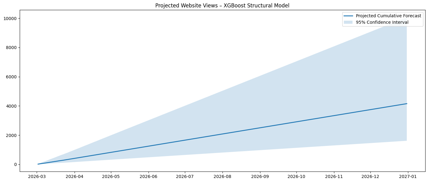
XGBoost
===Forecast totals===
01/03/2026 – 07/03/2026: 78
01/03/2026 – 31/03/2026: 393
01/04/2026 – 30/04/2026: 393
01/03/2026 – 31/05/2026: 823
01/01/2026 – 30/06/2026: 2,903
01/07/2026 – 31/12/2026: 2,501
01/01/2026 – 31/12/2026: 5,417
Results
Here are the current models that I am caching for the near future:
- Model 1: Auto-updating SARIMAX parameters
- Model 2: Log Views
- Model 3: Google Analytics
- Model 4: Prophet
- Model 5: XGBoost
From the analysis that I have completed, it has concluded that both of the following models should continue to be preferred over the others:
- Model 1: Auto-updating SARIMAX parameters
- Model 3: Google Analytics
This is due to their forecasted values (views) being the best suited based on the confidence interval range across the various measures (week, current month, next month, etc). Here is a summary of those findings:
Dataset
| Model | Value | CI Upper | CI Lower | Range | |
| Week | 1 | 139.9 | 50.9 | 229.0 | 178 |
| Current month | 1 | 646.4 | 587.1 | 705.6 | 119 |
| Next month | 1 | 97.4 | 38.1 | 156.6 | 119 |
| Next 3 months | 1 | 1634.8 | 617.3 | 2652.2 | 2035 |
| First 6 month | 1 | 4561.7 | 2458.5 | 6664.9 | 4206 |
| Last 6 months | 1 | 6611 | 3199.9 | 16774.0 | 13574 |
| Full year | 1 | 11173.0 | 4385.9 | 17960.0 | 13574 |
| Week | 2 | 109.2 | 20.6 | 491.4 | 471 |
| Current month | 2 | 619.1 | 602.9 | 687.3 | 84 |
| Next month | 2 | 20.1 | 3.9 | 88.3 | 84 |
| Next 3 months | 2 | 1134.5 | 195.2 | 5491.2 | 5296 |
| First 6 month | 2 | 3495.5 | 1590.8 | 13018.6 | 11428 |
| Last 6 months | 2 | 3399 | 688.5 | 36481.0 | 35793 |
| Full year | 2 | 6894.2 | 1924.5 | 37717.0 | 35793 |
| Week | 3 | 86.3 | 35.2 | 201.0 | 166 |
| Current month | 3 | 614.9 | 605.5 | 635.8 | 30 |
| Next month | 3 | 0.0 | 0.0 | 0.0 | |
| Next 3 months | 3 | 811.2 | 328.5 | 1894.0 | 1566 |
| First 6 month | 3 | 2912.0 | 1915.1 | 5147.9 | 3233 |
| Last 6 months | 3 | 2506.0 | 1015.9 | 5847.9 | 4832 |
| Full year | 3 | 5431.7 | 2936.6 | 11027.7 | 8091 |
| Week | 4 | 86.3 | 35.2 | 201.0 | 166 |
| Current month | 4 | 614.9 | 605.5 | 635.8 | 30 |
| Next month | 4 | 0.0 | 0.0 | 0.0 | |
| Next 3 months | 4 | 811.2 | 328.5 | 1894.0 | 1566 |
| First 6 month | 4 | 2912.0 | 1915.1 | 5147.9 | 3233 |
| Last 6 months | 4 | 2506.0 | 1015.9 | 5847.9 | 4832 |
| Full year | 4 | 5431.7 | 2936.6 | 11027.7 | 8091 |
| Week | 5 | 91.2 | 35.9 | 219.9 | 184 |
| Current month | 5 | 614.8 | 605.2 | 637.0 | 32 |
| Next month | 5 | 0.0 | 0.0 | 0.0 | |
| Next 3 months | 5 | 5605.8 | 2942.2 | 11793.4 | 8851 |
| First 6 month | 5 | 2912.0 | 1915.1 | 5147.9 | 3233 |
| Last 6 months | 5 | 2506.0 | 1015.9 | 5847.9 | 4832 |
| Full year | 5 | 5431.7 | 2936.6 | 11027.7 | 8091 |
Preferred model based on the minimum average confidence interval range (across all measures):
Model: 3 – Google Analytics
| Model Number | Average Range Value | Model Name |
| 1 | 4,829 | Auto-updating SARIMAX parameters |
| 2 | 12,663 | Log Views |
| 3 | 2,986 | Google Analytics |
| 4 | 2,990 | Prophet |
| 5 | 5,385 | XGBoost |
Preferred model based on the lowest CI range (across all measures):
| Measure | CI Range | Model Number | Model Name |
| Week | 165.8 | 2 | Log Views |
| Current month | 30.3 | 3 | Google Analytics |
| Next month | 84.4 | 2 | Log Views |
| Next 3 Months | 1,565.5 | 3 | Google Analytics |
| First 6 months | 3,232.8 | 3 | Google Analytics |
| Last 6 months | 4,832 | 3 | Google Analytics |
| Full year | 8,091.1 | 3 | Google Analytics |
Preferred model based on the maximin maximin principle; maximise the output for the minimised cost (greatest forecasted value for each measure based on the minimised confidence interval):
| Measure | Forecasted Value | Model Number | Model Name |
| Week | 86.3 | 2 | Log Views |
| Current month | 614.9 | 3 | Google Analytics |
| Next month | 20.1 | 2 | Log Views |
| Next 3 Months | 811.2 | 3 | Google Analytics |
| First 6 months | 2,912 | 3 | Google Analytics |
| Last 6 months | 2,506 | 3 | Google Analytics |
| Full year | 5,431.7 | 3 | Google Analytics |
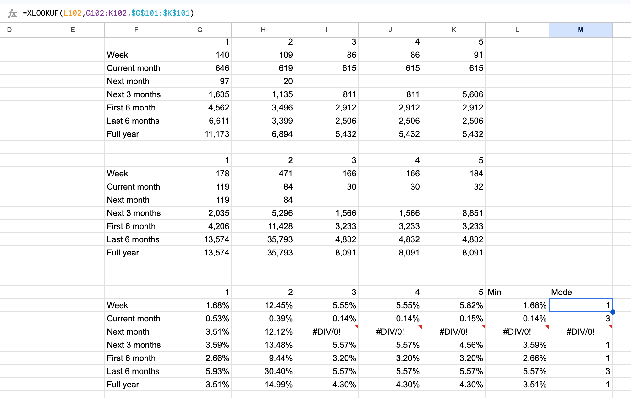
When considering the numbers above, it doesn’t take into account the scale of those values over the confidence interval ranges, relative to each measure:
| Measure | 1 | 2 | 3 | 4 | 5 | Minimum | Model |
| Week | 1.68% | 12.45% | 5.55% | 5.55% | 5.82% | 1.68% | 1 |
| Current month | 0.53% | 0.39% | 0.14% | 0.14% | 0.15% | 0.14% | 3 |
| Next month | 3.51% | 12.12% | 3.51% | 1 | |||
| Next 3 Months | 3.59% | 13.48% | 5.57% | 5.57% | 4.56% | 3.59% | 1 |
| First 6 months | 2.66% | 9.44% | 3.20% | 3.20% | 3.20% | 2.66% | 1 |
| Last 6 months | 5.93% | 30.40% | 5.57% | 5.57% | 5.57% | 5.57% | 3 |
| Full year | 3.51% | 14.99% | 4.30% | 4.30% | 4.30% | 3.51% | 1 |
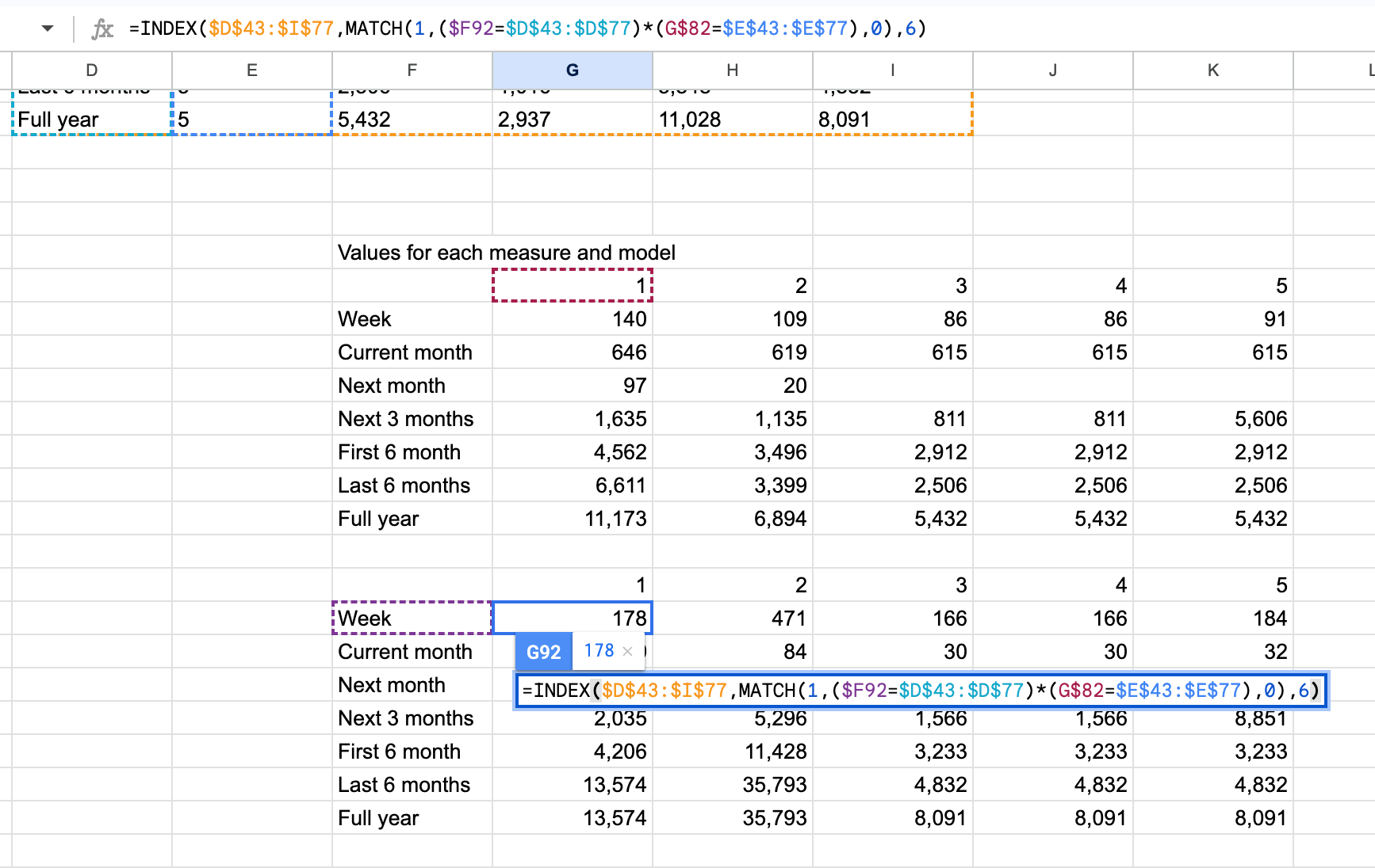
Each model’s cell possess the Coefficient of Variation (CV) divided by the model-measure’s value:
=(Confidence Interval/2)/SQRT(DAYS360(“01/01/2023″,”31/12/2026”))/Measure Value
The table above was derived by:
=INDEX($D$43:$I$77,MATCH(1,($F83=$D$43:$D$77)*(G$82=$E$43:$E$77),0),3)
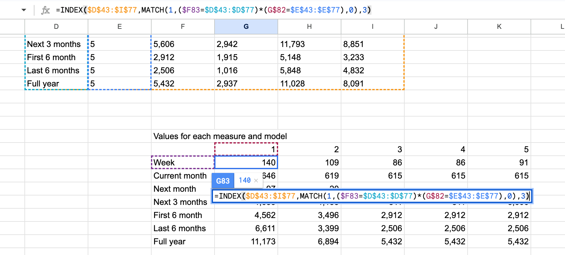
=INDEX($D$43:$I$77,MATCH(1,($F92=$D$43:$D$77)*(G$82=$E$43:$E$77),0),6)
Conclusion
Although I have statistical evidence for the models that I’ll be following, I have decided that I’ll be running the following in parallel:
- Model 1: Auto-updating SARIMAX parameters
- Model 3: Google Analytics
- Model 4: Prophet
- Model 5: XGBoost
Model 3 requires a bit more automation to be completed, specifically funneling the daily Google Analytics into the file that holds the WordPress data, processing them together.
