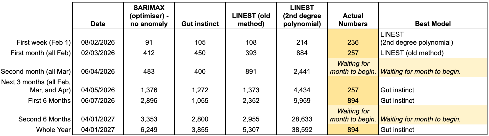
Last week, I provided an update for how my models were performing against human behaviour. Within that post, I included a decision-making table that automatically tells me which model I should be favouring during certain periods:

What I wanted to showcase was how I went creating this process, but also to do one of those things that I’ve previously preached — document a sequence of events that I know I’ll forget in the future, but have a resource to back up my thinking. Speaking of backing up, I should probably start to think about a long-term solution for my NAS and Plex solution.

Processes Documentation

Automated LINEST Function

I’ll get to the table (above) a little farther down, but a core part of the table are the LINEST models that I use. For those who are versed in differences between Excel and Google Sheets, you’ve probably discovered the ease in Google Sheets’s handling of entire columns data ranges $A$2:$A vs $A$2:$A$135. For those who aren’t aware of this difference, can you see the problem? I’m going to apply this to the context of automating the dynamic dataset to a LINEST function.

As a brief summary, this LINEST function provides you with the x and c output of the y=mx+c function with your provided y and x variables. As you collect more data for this model, you need to adjust the dataset length otherwise the function errors when attempting to parse empty cells:

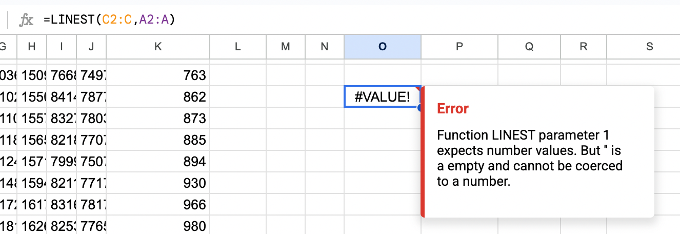
To resolve this, there are a few suggested approaches to circumvent this problem:

• Named Ranges

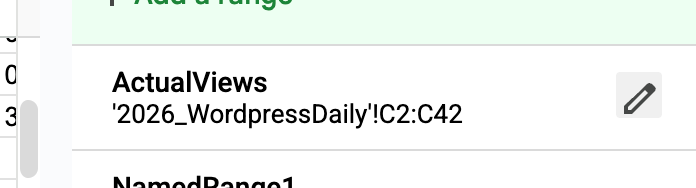
Whilst trying this solution, I was unable to set the Named Range for ‘ActualViews’ as dynamic, i.e. C2:C; it would always resolve to the data’s last value’s row, in this case (C42).

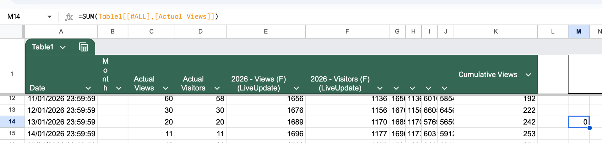
• Tables

Not going to lie, I spent more time that I wanted in an attempt to get this working. My assumption is that I’m missing something very simple, but all peoples’ suggested solutions for this were not simple and ultimately incorrect:

• Using OFFSET and COUNTA (Dynamic Range)

I’m all for OFFSET and COUNTA, but when you integrate this into the formula, it starts to get a bit too messy:

=ARRAYFORMULA(LINEST(OFFSET(K$1,1,0,COUNTA(K:K)-1,1),OFFSET(A$1,1,0,COUNTA(A:A)-1,1)^{1,2},1,1))

• Using INDEX and MATCH (For Large Data Sets)

=LINEST(A2:INDEX(K:K,MATCH(9.99999999999999E+307,K:K)),A2:INDEX(A:A,MATCH(9.99999999999999E+307,K:K)))

I originally created this in my Excel Presentation portfolio file, specifically for calculation of Photovoltaic costs and recoup values:

=LINEST(Data!G3:INDEX(Data!G3:G,MATCH(B101,Data!G3:G)),Data!J3:INDEX(Data!K3:K,MATCH(B101,Data!G3:G)),1,1)

Where B101= 1E+308

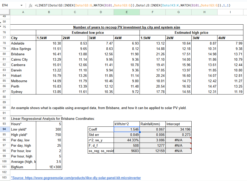
This method is essentially returning the row where the last data point exists and doesn’t error out due to the BigNum (B101) acting as an extremely large column value, filled with non-value values. But, there is a cleaner way to implement this solution.

• Using FILTER

For the linear LINEST model:

=ARRAYFORMULA(

LINEST(

FILTER(K2:K,K2:K<>“”,A2:A<>“”),

FILTER(A2:A,K2:K<>“”,A2:A<>“”),

1,1)

)

For the multi-degree polynomial LINEST model:

=ARRAYFORMULA(

LINEST(

FILTER(K2:K,K2:K<>“”,A2:A<>“”),

FILTER(A2:A,K2:K<>“”,A2:A<>“”)^{1,2},

1,1)

)

I argue that this is a cleaner method for implementing this solution, but only where the data is complete for both columns that you’re regressing on. If you have some dates within the dataset (not at the end) where they are blank, it will immediately filter out those incomplete points.

Best Model Automation Table

After accounting for these LINEST models automatically, we can utilise them in a summary table; the purpose for this post.

Date

I had set the dates up for ‘post date’ rather than actual testing date. Instead of manipulating the columns to fit these date ranges, I decided to use a SUMIF and essentially filtered by a date bucket. 

Model Values

All of these values have all been calculated using their own methods:

• SARIMAX is completed using Python,
• Gut instinct is based on my interpretation over time,
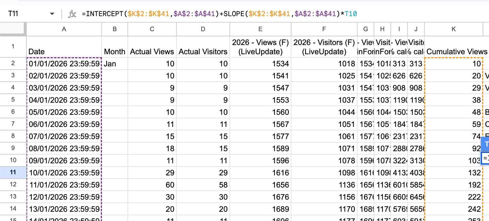
• LINEST (old method) is completed by creating an INTERCEPT()+SLOPE()*dateOfForecast formula, using specified cumulative view dates, where T10 = 08/02/2026:

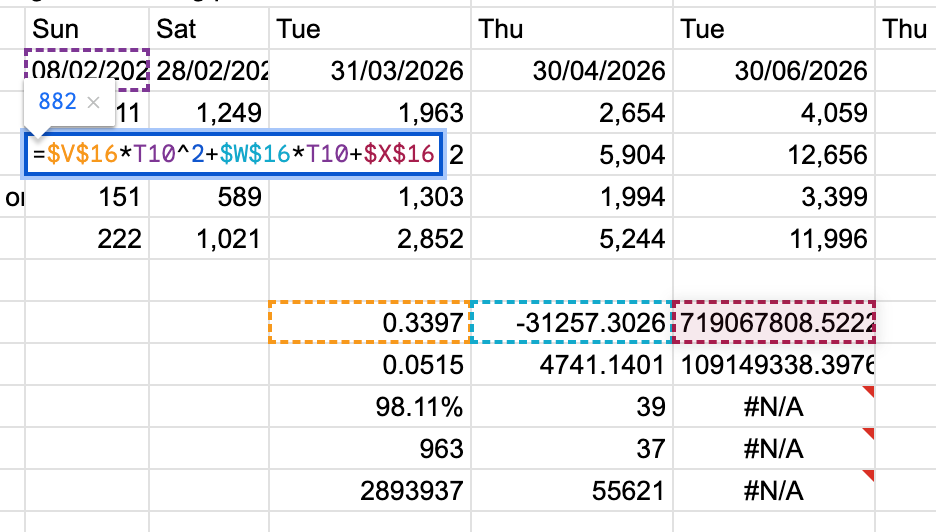
• LINEST (2nd degree polynomial) is the the same as (old method), but using a LINEST() function with static values:

=$V$16*T10^2+$W$16*T10+$X$16

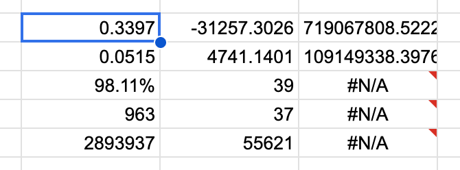
=ARRAYFORMULA(LINEST($K$2:$K$41,$A$2:$A$41^{1,2},1,1))

Actual Numbers

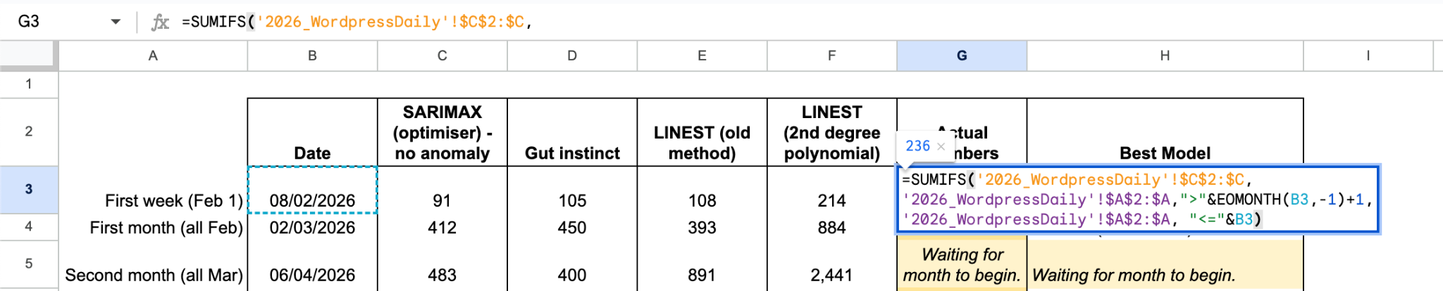
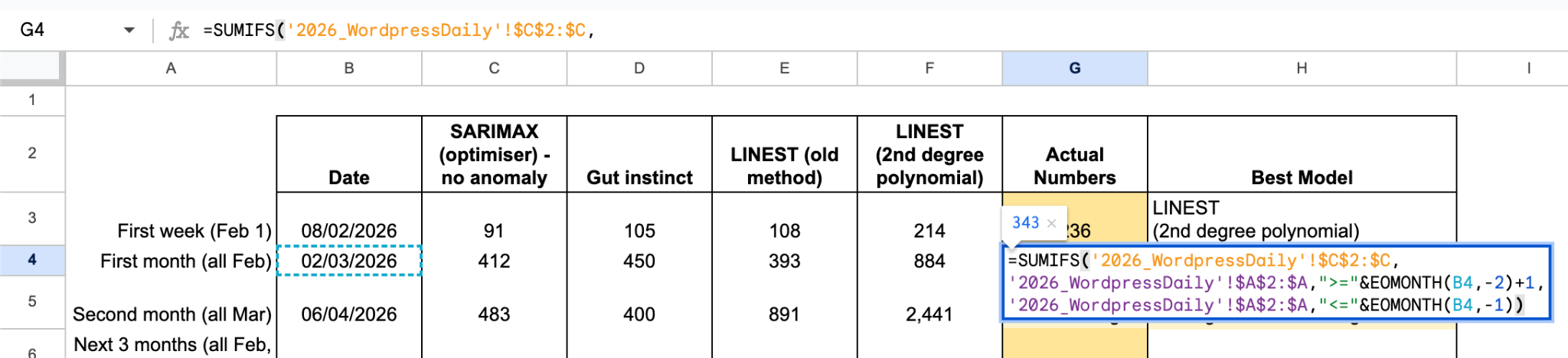
Each one of these formulas are about adjusting the “filters” in the SUMIFS function to create buckets for each timeframe that we’re calculating the views for. I’m interested in summing the views between 2nd February to 8th February. This is due to the logic that I can analyse the data on the morning of 9th February before hitting ‘Post’.

Calculating Actual Numbers Live:

=SUMIFS(‘2026_WordpressDaily’!$C$2:$C,

‘2026_WordpressDaily’!$A$2:$A,“>”&EOMONTH(B3,-1)+1,

‘2026_WordpressDaily’!$A$2:$A,“<=”&B3)

=SUMIFS(‘2026_WordpressDaily’!$C$2:$C,

‘2026_WordpressDaily’!$A$2:$A,“>”&EOMONTH(B3,-1)+1,

‘2026_WordpressDaily’!$A$2:$A,“<=”&B3)

=SUMIFS(‘2026_WordpressDaily’!$C$2:$C,

‘2026_WordpressDaily’!$A$2:$A,“>=”&EOMONTH(B4,-2)+1,

‘2026_WordpressDaily’!$A$2:$A,“<=“&B4,-1)

Best Model

=INDEX($C$2:$F$2,1,

MATCH(MIN(ABS($G3–$C3:$F3)),

ABS($G3–$C3:$F3),0))

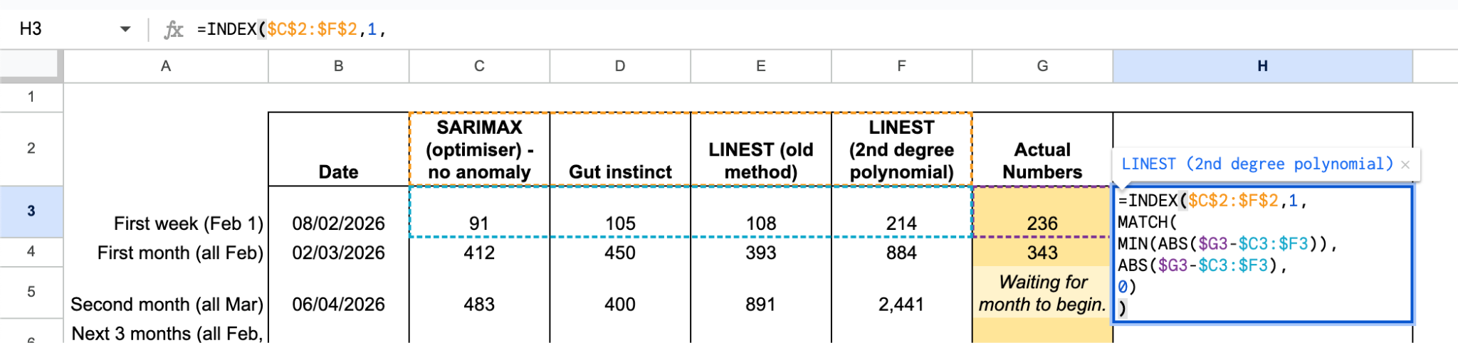
Measured all of the models and created an INDEX-MATCH to solve this problem. The model names are the reference as we want to see the ideal model’s name. Index’s second argument is asking for the row and since there’s only 1 row ($C$2:$F$2), we can simply place a 1 in here. The second argument is looking for the appropriate column. Ultimately, we’re looking to find the model with the closest value to the actual numbers; above or below doesn’t matter.

The following is MATCH’s function: MATCH(search_key, range, [search_type]).

Argument 2, the range, is what we want to observe are the current total views (G3) minus the values for each model ($C3:$F3). $G3-$C3:$F3 will provide you with an array of those values: 145; 131; 128; 22. We can now account for the models that over perform for the actual values by turning those negative values to positive using the ABS() function.

Argument 1, the search key, the smallest (MIN) value in the array of $G3-$C3:$F3 values that are now positive. We can wrap the range formula in a MIN() function to retrieve this value. We can now place a 0 in Argument 3 since we’re going to be reporting exact values.

In the case that the month in the analysis hasn’t started, (March or the last 6 months), we can wrap the whole function in an IFERROR() function:

=IFERROR(

INDEX($C$2:$F$2,1,

MATCH(MIN(ABS($G3–$C3:$F3)),

ABS($G3–$C3:$F3),0)),

“Waiting for month to begin.”)

Is there anything that you repeat over and over again without remembering how you landed on the solution?