In a previous post, I mentioned that I was responsible for tracking updates in timetables. This is somewhat of an extension of that post. I was thinking about what could happen to these groups of people after the grouping has been completed. What happens when you actually need to group people together. How do you do it? What is the angle? Do you ask them who they are best suited to? How reliable is that? What are you attempting to achieve? What is the metric to choose the pairings? …the mind wanders.

I thought about various ways that this type of pairing was possible, but I’ve considered an interesting approach, using personality types. One of my favourite personality tests is the Myers-Briggs, which I’ve spoken about in a recent post. It just so happens that the people I used in this previous post, I actually have their personality results at hand. I’m getting ahead of myself. Let me explain the process of what I’ve done and I can show you how I’ve matched people up according to their personality type. Importantly, not matching certain people based on their personality type.

The following is a shorthand version, and I’ll go into detail afterwards. ‘I created a list of 15 people. 10 of those people would be chosen to join the group and 5 would not be invited. I then created a group matching operation in Excel. I looked at a particular date of interest, e.g. 19th March, and compared it to previous dates, e.g. 4th March, 5th March, etc, to see the percentage of people in that day’s group that were previously assigned the future date (19th March). The higher the resulting percentage (of those 10 who were chosen) means the fewer potential reassignments (of the 5 reserve people) I would have had to have done for the 13th March day I was originally looking at.’

Let’s go through step by step.

https://docs.google.com/spreadsheets/d/1ewDyMtCbMoa0Vr81MHCTEfA7I8yte72L5BSj9On0Lfo/edit?gid=0#gid=0

Here is the order of things, in case you’d like to skip ahead:

1. Assigned Groups
2. Matching Individuals in Groups
   1. Finding who is present
   2. Percentage Calculation
3. How to Match Personalities
   1. Initial VLOOKUP
   2. Searching for the Matching and Non-Matching Personalities
   3. Full Formula
   4. Formula Broken Down
   5. Calculation Formula Explained
   6. Matching People with the Formula
4. Python
   1. Scaling with Python
   2. Algorithm

Assigned Groups

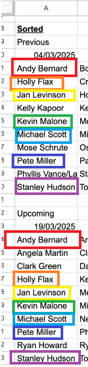
Here are the different types groups; those that have been previously assigned, allocated, and completed (4th March – 6th March):

Here are the upcoming event groups; those that are yet to be finalised (19th March – 21st March):

In reality, I would have about 30 groups to confirm; 10 future events to confirm based on 20 previous ones. This would be 200 (10*20) iterations that I need to cycle through. To best do this, computationally and for quick visual referencing, I sorted all groups alphabetically:

=SORT(A4:A13,1,1)

Matching Individuals in Groups

Next was to find the number of same people in future groups that are present in previous groups (D57:F57). I performed this process to reduce the cognitive load of potential pairing calibration. If there is a certain percentage of people (D58:F58) in a future group that have been present in a previously (finalised) group (D59:F59), this implies that there is only a small amount of considered pairing process required based on personality types:

What I need to do is figure out if some people in the upcoming 19/03/2025 session were also in the 04/03/2025 session:

=ARRAYFORMULA(IF($A$31:$A$40<>“”,IFERROR(MATCH($A$31:$A$40,A44:A53,0),“”),“”))

Here are the people who match between the days:

Finding who is present

This will output an indexed number that shows if a person in the future date exists in the previous date. If a person doesn’t exist previously, no output is generated:

Since the formula is attempting to match those in the previous dates to the future ones, we will see an output of numbers for those people in the future that are present in the past. So, during this word logic, look at the past date (04/03/2025) first. Can you see the person in the future date in the past group? Then, this person will show up in this output with an index number between 1 and 10 (aligned to this future date group). If they aren’t in the future group, they will have no output (blank):

1. Andy Bernard was in the past group, position 1, and is also present in the future group (position 1). We see an index of 1, his position in the future group,
2. Holly Flax was in the past group, position 2, and is also present in the future group (position 4). We see an index of 4, her position in the future group,
3. Jan Levinson (no Gould) was in the past group, position 3, and is also present in the future group (position 5). We see an index of 5, her position in the future group,
4. Kelly Kapoor was in the past group, position 4, but is not present in the future group. We see no indexed number,
5. Kevin Malone was in the past group, position 5, and is also present in the future group (position 6). We see an index of 6, hs position in the future group,
6. Michael Scott was in the past group, position 6, and is also present in the future group (position 7). We see an index of 7, hs position in the future group,
7. Mose Schrute was in the past group, position 7, but is not present in the future group. We see no indexed number,
8. Pete Miller was in the past group, position 8, and is also present in the future group (position 8). We see an index of 8, hs position in the future group,
9. Phyllis Vance/Lapin was in the past group, position 9, but is not present in the future group. We see no indexed number,
10. Stanley Hudson was in the past group, position 10, but is not present in the future group. We see no indexed number.

This means that we have 3 people that we need to consider with pairings: Angela Martin, Clark Green, and Ryan Howard.

Percentage Calculation

I can now perform a percentage calculation of all existing indexes divided by the number of all people in the previous group. Again, the higher the percentage, the more of these people existed in the list on the previous date’s day. This means it requires less mental accounting for personality pair matching. The lower the percentage means I need to consider more people (and personalities) to match. To calculate this, I created the following formula:

=COUNTIF(D59:D68,“>0”)/COUNTA(A44:A53)

Yes, I could have easily entered /10, but I like to keep this option open for future automation, especially if someone is removed from this list and that denominator value is not changed from a 10 to a 9. This formula counts the number of discrete values that are greater than 0 in this matching (indexed) list. There are 7 out of 10 matches; which lines up with those 3 people (above) that we need to account for.

Now that this first date is complete, I can drag this formula across and observe how many people exist in these other past dates, in comparison to 19/03/2025:

Across these three dates, it’s advantageous for me to base my initial pairing analysis on the 4th March. As a corollary, this is because it has the highest percentage of matching against any of the other dates.

How to Match Personalities

This is where manual work would begin of analysing each individual day and the people that occupy it. I can observe the participants within each day, consider their personalities, then match accordingly. Although it’s possible to do this for a single day, then comparing them across 30, it can become cognitively taxing. Especially if there are some factors where you hold knowledge, or intuition, and you carry the load of bearing that information. This is where we can integrate an additional dataset, assisting us in making connections and decisions.

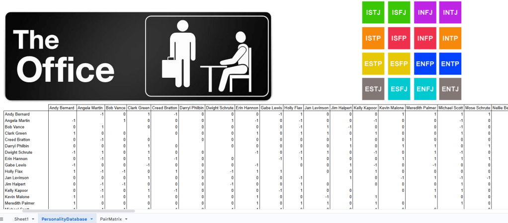
I was able to come across The Office personality indicators online. I’m thinking about this from the perspective of both (logic, Venn diagrams, and SQL) inner joins and outer joins. I’m interested in considering two modes simultaneously; which personalities work well together and which personalities do not work well together. I created a PersonalityDatabase sheet and entered the data:

My intention here is to create a matrix that shows how all people are related to one another through their personalities. This is similar to the correlation matrix that I created in the collusion post in July last year. This matrix will act as a big lookup database and allow all the user to easily match people together. Here is a sample of what I’m going to create, but I’ll slowly step through the logic for how I got there:

Initial VLOOKUP

Let’s consider this dataset. I can use a VLOOKUP to pull a person’s MBTI Type:

=VLOOKUP(F6,$A$6:$B$31,2,0)

I can use the same function to pull another person’s MBTI Type:

=VLOOKUP(H6,$A$6:$B$31,2,0)

The data includes a list of MBTI Types that a person Works Well With and Doesn’t Work Well With, separated by commas. There’s two approaches that I could take here; 1. separating the cells by their comma delimiter, or 2. using the SEARCH() function for for the cell:

To start with, we’re going to need two VLOOKUP functions. I’ll work my way from the outer VLOOKUP in. I want to search for Michael’s MBTI Type in Erin’s Works Well With cell. So, the VLOOKUP search_key is Michael’s MBTI Type, which could be located somewhere in the cell, hence the wildcards. Now, I want to use Erin’s ‘Works Well With’ cell (column 3), but I need to account for the fact that it may not be Erin. So, I will use the nested VLOOKUP function to find whomever is entered into F6. Since there is only 1 column, I am going to return column 1.

All I want to know in this output is whether they work well together and not the personalities that they can work well with. For this, I’m going to come up with my own definitions, which I will be using in greater detail later:

Works Well Together: 1

Does Not Work Well Together: -1

Neutral: 0

Self: <blank>

Searching for the Matching and Non-Matching Personalities

This is where I can use SEARCH and VLOOKUPs. Search looks for the final VLOOKUP output key term in I6 and returns the index value where it is located. We can see that Michael’s MBTI Type is the first entry in Erin’s Works Well Together cell:

We can then wrap this in an ISNUMBER function for a TRUE or FALSE response:

=ISNUMBER(SEARCH(I6,VLOOKUP(“*”&I6&“*”,VLOOKUP(F6,Table1,3,0),1,0)))

We can do the same for the Doesn’t Work Well Together, but change the inner VLOOKUP column to 4:

=ISNUMBER(SEARCH(I6,VLOOKUP(“*”&I6&“*”,VLOOKUP(F6,Table1,4,0),1,0)))

Full Formula

This is the core mechanic for how I built the broader matrix. I’ll break down the formula variable by variable then show how it’s all related:

=LET(horizSearch,

VLOOKUP(G$39,$A$6:$B$31,2,0),

vertSearchPos,

VLOOKUP($F40,$A$6:$B$31,3,0),

vertSearchNeg,

VLOOKUP($F40,$A$6:$B$31,4,0),

positive,

SEARCH(horizSearch,vertSearchPos),

negative,

-SEARCH(horizSearch,vertSearchNeg),

IF(G$39=$F40,,IFERROR(IFERROR(IF(positive>0,1,0),IF(negative<0,-1,0)),0)))

Formula Broken Down

The first variable, horizSearch, returns the person located in row 40’s MBTI Type:

=LET(horizSearch,

VLOOKUP(G$39,$A$6:$B$31,2,0),

vertSearchPos returns the Works Well With array of the people located in column F:

vertSearchPos,

VLOOKUP($F40,$A$6:$B$31,3,0),

vertSearchNeg returns the Doesn’t Works Well With array of the people located in column F:

vertSearchNeg,

VLOOKUP($F40,$A$6:$B$31,4,0),

This is where the definitions that we mentioned before come in. Using the variables that we created before, horizSearch and vertSearchPos, we use SEARCH() to determine whether the person in question’s MBTI type is located within another person’s MBTI Works Well With array. If they do, then it returns a positive value:

positive,

SEARCH(horizSearch,vertSearchPos),

Just like positive, we’re now looking for a match for those who do not work well together:

negative,

-SEARCH(horizSearch,vertSearchNeg),

Calculation Formula Explained

We account for a few cases in this formula:

IF(G$39=$F40,,IFERROR(IFERROR(IF(positive>0,1,0),IF(negative<0,-1,0)),0)))

I’ll replace this formula’s variables with numbers to make it a little easier to explain:

IF(<1>,,IFERROR(IFERROR(IF(<2>,1,0),IF(<3>,-1,0)),0)))

<1>: We have dealt with this in a previous post, where we want to ignore people on the diagonal of the matrix. So, where the person in the row is the same as the person in the column, the output is blank,

<2>: We are testing whether the relationship between the two people is a good working relationship. If so, then there is a 1 that is returned,

<3>: We are testing whether the relationship between the two people is not a positive working relationship. If so, then there is a -1 that is returned, otherwise, they are neutral/indifferent with one another,

IF(<1>,,IFERROR(<5>,<4>))

<4>: Since we are using VLOOKUP to search for this information, this function throws an error when there is no match. We need to account for these errors and we can do that by using IFERROR. The inner IFERROR (4) is looking for the base case of, ‘is this positive value?’ If not, then the error is thrown, so we account for the negative value (case) in the second argument.

<5>: The outer IFERROR (5) is now detecting for neither the positive nor the negative, which is the neutral/indifferent cases. If these exist, then a 0 is produced.

Matching People with the Formula

Now that we have this database, we can start to utilise it in production. I’ll create one last sheet, PairMatrix, to demonstrate how it can be utilised:

I’ll start by putting a date field in the sheet:

I’ll import the the data from Sheet 1, where the groups have been created, and filter them based on this date:

=FILTER(Sheet1!A4:C13,Sheet1!A3:C3=B2)

Next, I’ll create a dropdown list of names from the people that are located in the database on this sheet:

Finally, we can create the ‘Pairs with’ and ‘Does Not Pair’ columns, based on the data and assigned personality matching values. For those who pair, we want to filter all of the names in column F based on whether the person in B3 has an aligned personality, i.e. a value of 1:

=FILTER(F11:F20,INDEX(G11:P20,F11:F20,MATCH(B3,G10:P10,0))>0)

For those who do not pair, we want to perform the same lookup, except look for negative values:

=FILTER(F11:F20,INDEX(G11:P20,F11:F20,MATCH(B3,G10:P10,0))<0)

We can now do quick search and match people together in pairs:

What I find interesting about some of these pairings is that it makes you reflect on the show’s storylines and actually dig even deeper into the motivations of the characters, e.g. Michael Scott pairing well with Toby Flenderson. Says more to Michael’s psyche than his potential working ability with Toby.

Python

Scaling with Python

Although the example is a small and manageable number of pairings to consider, this process sees its benefits at scale. If this is the case, and I was going to maintain this process in Excel, I would definitely be transitioning to an INDEX-MATCH-MATCH formula as it scales much better than VLOOKUP. There’s an issue with this approach though for matching pairs together. You need to step through everything, one person at a time. What we need to do is automate this part of the manual process and we can do that using Python.

Algorithm

Within Operations Research, you can solve this matching problem by using the Hungarian Algorithm (Kuhn-Munkres Algorithm). This is usually used for assignment problems, which I’ve actually explored in a previous optimisation post.

Python code

import numpy as np

from scipy.optimize import linear_sum_assignment

# Given matrix (excluding headers)

match_matrix = np.array([

    [0, -1, 0, 0, 1, 1, 0, 1, 0, 0],

    [0, 0, -1, 0, 1, 1, 1, 1, 1, 0],

    [-1, -1, 0, 0, -1, -1, 0, -1, 0, 0],

    [0, 0, 0, 0, -1, -1, -1, -1, -1, 0],

    [1, 1, -1, -1, 0, 0, 0, 0, 0, 0],

    [1, 1, -1, 0, 0, 0, 0, 0, 0, 0],

    [1, 1, -1, 0, 0, 0, 0, 0, 0, 0],

    [1, 1, -1, -1, 0, 0, 0, 0, 0, 0],

    [1, 1, -1, 0, 0, 0, 0, 0, 0, 0],

    [0, 0, 0, 0, 0, 0, 0, 0, 0, 0]

])

# List of names

names = [“Kelly Kapoor”, “Andy Bernard”, “Stanley Hudson”, “Jan Levinson”, “Mose Schrute”,

         “Holly Flax”, “Michael Scott”, “Kevin Malone”, “Pete Miller”, “Phyllis Vance/Lapin”]

# Convert to a cost matrix (since Hungarian algorithm minimizes, negate values)

cost_matrix = -match_matrix

# Set self-matching penalties (large positive number instead of negative)

np.fill_diagonal(cost_matrix, 99999)

# Solve assignment problem

row_ind, col_ind = linear_sum_assignment(cost_matrix)

# Track assigned people to avoid double-pairing

paired = set()

optimal_pairs = []

# First pass: Assign best possible pairs while avoiding duplicates

for i, j in zip(row_ind, col_ind):

    if i != j and i not in paired and j not in paired:

        optimal_pairs.append((names[i], names[j]))

        paired.add(i)

        paired.add(j)

# Find any unpaired individuals

unpaired = [names[i] for i in range(len(names)) if i not in paired]

# If two people are left, pair them

if len(unpaired) == 2:

    optimal_pairs.append((unpaired[0], unpaired[1]))

# Print results

for pair in optimal_pairs:

    print(pair)

So, providing the code with day one data, we have the output of the following pairs:

1. Kelly Kapoor, Mose Schrute
2. Andy Bernard, Holly Flax
3. Stanley Hudson, Jan Levinson
4. Kevin Malone, Phyllis Vance/Lapin
5. Michael Scott, Pete Miller

Based on the data that has been provided, this pairing all makes sense and is sound. Based on the show, I’m not too sure:

Source: https://i.redd.it/1zc9czyt69k61.png