Back in October of this year (2024), I made a post about using an ARIMA Stock Market Predictor Model in Python. Today is an update of that predictor. This is essentially what data, science, and learning is all about, right? Reviewing and updating previous notions or ideas; see more in the continuing BPM series over the next few weeks. After reviewing this code, I’ve made the following updates to it, included it in this post and the .ipynb file here.

Key Enhancements:

1. Stationarity Check and Differencing: I have included an extra stationarity test (ADF) and applied differencing, where it’s deemed to be necessary,to stabilise the mean.
2. p-value Handling: In the case of insignificant p-values, this code adjusts the data by removing all non-significant parameters. This improves the overall model’s accuracy and simplicity.
3. Automatic Akaike Information Criterion (AIC) Minimization: Reducing the manual specifications of the ARIMA parameters, pmdarima’s auto_arima can automate these specifications. By analysing the AIC and BICs of each iteration, it selects the best model and tests for stationarity.
4. More Detailed Investment Analysis: In the previous model, I believe that there was too much qualitative information, providing each investor profile type. I have included clearer signals, using confidence intervals, and integrating risk factors.
5. Graphical Outputs: Linked with 4, I have included clearer investor profile signals, i.e. buy, sell, or hold, based on forecast intervals and z-scores.

import yfinance as yf

import statsmodels.api as sm

import matplotlib.pyplot as plt

from statsmodels.tsa.arima.model import ARIMA

from statsmodels.tsa.stattools import adfuller

import pandas as pd

import numpy as np

import itertools

from scipy.stats import norm

import pmdarima as pm

import time

from datetime import timedelta

import warnings

warnings.filterwarnings(“ignore”)

# Fetch stock data

def fetch_stock_data(ticker, period=’1d’, interval=’1m’):

    stock_data = yf.download(ticker, period=period, interval=interval)

    stock_data.index = pd.to_datetime(stock_data.index)

    stock_data = stock_data.asfreq(‘T’)  # Setting frequency to minute

    return stock_data[‘Close’]

ticker = ‘AAPL’

stock_prices = fetch_stock_data(ticker)

display(stock_prices)

# Check for stationarity and apply differencing if necessary

def check_stationarity(series):

    result = adfuller(series.dropna())

    print(f’ADF Statistic: {result[0]}’)

    print(f’p-value: {result[1]}’)

    if result[1] > 0.05:

        print(“Series is non-stationary, differencing required.”)

        return series.diff().dropna()  # Differencing if needed

    else:

        print(“Series is stationary.”)

        return series

stock_prices = check_stationarity(stock_prices)

# Use auto_arima to find the best model based on AIC/BIC

def auto_arima_model(stock_prices):

    model = pm.auto_arima(stock_prices, seasonal=False, stepwise=True, suppress_warnings=True)

    print(f”Selected ARIMA Order: {model.order}”)

    return model

arima_model = auto_arima_model(stock_prices)

# Forecast prices with the ARIMA model

def forecast_prices(model, steps=10):

    forecast = model.predict(n_periods=steps, return_conf_int=True)

    forecast_values, conf_int = forecast

    return forecast_values, conf_int

forecast_values, conf_int = forecast_prices(arima_model, steps=10)

# Investment Analysis

def analyse_investment(stock_prices, forecast_values, conf_int):

    recent_volatility = np.std(stock_prices[-30:])  # Last 30 minutes

    recent_return = stock_prices.pct_change().mean()

    forecast_mean = np.mean(forecast_values)

    forecast_std = np.std(forecast_values)

    recent_price_change = stock_prices.pct_change()[-30:]

    z_scores = (recent_price_change – recent_price_change.mean()) / recent_price_change.std()

    buy_signals = z_scores < -2

    sell_signals = z_scores > 2

    print(“\nInvestment Analysis:”)

    # Risk-Taker

    print(“\nRisk-Taker:”)

    print(f”Volatility: {recent_volatility:.2f}, Return: {recent_return:.2%}”)

    print(f”Forecast Mean: {forecast_mean:.2f}, Forecast Std: {forecast_std:.2f}”)

    print(f”Buy Signals: {buy_signals.sum()} times, Sell Signals: {sell_signals.sum()} times”)

    # Risk-Neutral

    print(“\nRisk-Neutral:”)

    print(“Balanced risk-reward scenario.”)

    # Risk-Averse

    print(“\nRisk-Averse:”)

    print(“Consider safer investments due to uncertainty.”)

analyse_investment(stock_prices, forecast_values, conf_int)

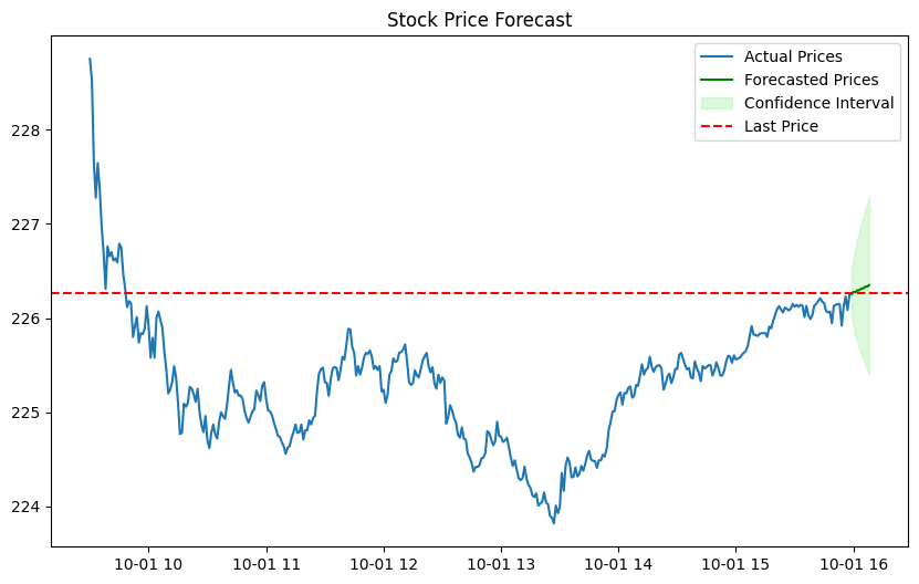
# Plot forecast with confidence intervals

def plot_forecast(stock_prices, forecast_values, conf_int, steps=10):

    plt.figure(figsize=(10, 6))

    plt.plot(stock_prices.index, stock_prices, label=’Actual Prices’)

    future_dates = pd.date_range(stock_prices.index[-1], periods=steps, freq=’T’)

    plt.plot(future_dates, forecast_values, label=’Forecasted Prices’, color=’green’)

    plt.fill_between(future_dates, 

                     conf_int[:, 0], conf_int[:, 1], 

                     color=’lightgreen’, alpha=0.3, label=’Confidence Interval’)

    plt.axhline(stock_prices[-1], color=’red’, linestyle=’–‘, label=’Last Price’)

    plt.title(‘Stock Price Forecast’)

    plt.legend()

    plt.show()

plot_forecast(stock_prices, forecast_values, conf_int)

# Live feed update

def live_feed(ticker, interval=60, steps=10):

    while True:

        stock_prices = fetch_stock_data(ticker)

        arima_model = auto_arima_model(stock_prices)

        forecast_values, conf_int = forecast_prices(arima_model, steps)

        plot_forecast(stock_prices, forecast_values, conf_int, steps)

        analyse_investment(stock_prices, forecast_values, conf_int)

        time.sleep(interval)

live_feed(ticker, interval=60, steps=10)

Is there something in here that you liked? Is there something not included that you think should be? Have you already made adjustments to the last post’s code and made it your own? Link it to the bottom and let me know what’s been happening on your end!