James Miller CV

1. Learn the fundamentals of Statistics
2. Learn SQL
3. Learn Python for Data Analysis
4. Learn Data Manipulation and Visualisation
5. Learn Learn Statistical Analysis
6. Learn Data Visualisation Tools
7. Work on Projects
8. Learn Data Storytelling

Statistical analysis stands as a cornerstone in the journey of data analysis, serving as a pivotal force in extracting meaningful insights and aiding informed decision-making. Positioned as the quantitative backbone, it empowers analysts and data scientists to derive reliable predictions and conclusions.

This type of analysis furnishes the necessary tools for describing and summarising data. You will be able to peruse my understanding of descriptive statistics in a previous post throughout this roadmap. These aspects of statistics offer a succinct portrayal of central tendencies and variabilities within the data. This facilitates a comprehensive understanding of the overall data characteristics, facilitating effective communication of findings to stakeholders.

Furthermore, statistical inference, a critical facet of this analysis, enables the extrapolation of predictions and conclusions about a population from a sample dataset—a crucial approach when analysing impractically large datasets. Techniques such as hypothesis testing and confidence intervals play a key role in assessing the reliability of findings, safeguarding against inaccurate or biassed conclusions.

The deployment of statistical models is equally crucial for unravelling intricate patterns and relationships within the data landscape. Regression analysis, for instance, serves to uncover the strength and nature of associations between variables, enabling predictive modelling and the understanding of various factors’ impacts on outcomes.

Moreover, statistical analysis becomes indispensable in decision-making scenarios fraught with uncertainty. Probability distributions and Bayesian methods offer a structured framework for quantifying and managing uncertainty, empowering analysts to make well-informed decisions even in the face of incomplete information.

A mastery of statistical analysis is pivotal within the data analysis roadmap. It equips professionals with the essential tools to articulate data descriptions, draw inferences, construct models, and navigate decision-making in uncertain environments. Devoid of a robust statistical foundation, data analysis risks subjectivity and unreliability, impeding the extraction of valuable insights from intricate datasets.

I propose that this following example of work, based on The Tennessee Study of Class Size in the Early School Grades by Frederick Mosteller in 1995, showcases how aspects of my understanding of Statistical Analysis have been developed throughout this journey. The data from the Project STAR: A Randomised Experiment of the Impact of Class Size Reductions on Pupil Achievement, is based on a 4-year experiment in Tennessee designed to evaluate the effect of class size on learning. Each participating school had at least one control group class and one treatment group.

Within Statistics, and ultimately Econometrics, Ordinary Least Squares Linear Regression analysis is a foundation tool that is used to model and understand the relationships between variables. However, there are some assumptions that need to be held before analysing a dataset.

Assumptions:

1. Linearity: The relationship between the independent variable X and the dependent variable Y is linear.

Y = β₀​ + β_1​X + ε

Example: In predicting house prices, assuming a linear relationship means that a change in square footage or the number of bedrooms has a constant effect on the house price. For instance, if a house with 1,000 square feet is $200,000, a house with 2,000 square feet is expected to be $400,000 under the linear assumption.

2. Independence: The residuals (ε) are independent of each other.

Cov(ε_i,ε_j) = 0 for i ≠ j

Example: In a study measuring the effectiveness of a new drug, the outcomes of different patients should be independent. The response of one patient to the drug should not influence the response of another patient.

3. Homoscedasticity: The variance of the residuals is constant across all levels of the independent variable 

Var(ε_i) = σ²

Example: Consider predicting student test scores based on the number of hours spent studying. Homoscedasticity implies that the variability in test scores should be consistent across all levels of study hours. In other words, the spread of residuals should be roughly constant.

4. Normality of Residuals: The residuals (ε) are normally distributed.
   1. This assumption is not required for estimation of coefficients but is useful for hypothesis testing and confidence intervals.

Example: Suppose you are modelling the sales of a product. While normality is not strictly necessary for parameter estimation, if the residuals are normally distributed, it allows for more accurate hypothesis testing and confidence interval estimation. This assumption is often tested through residual plots or statistical tests.

5. No Perfect Multicollinearity: There should not be perfect linear relationships among the independent variables.

Var(ε_i​) = σ² (constant)

Example: Imagine predicting a person’s income based on both their education level and the number of years of work experience. If these two predictors are perfectly correlated (e.g., someone with more education tends to have more work experience), it can cause issues in estimating the individual contributions of each variable.

This project is concerned with Random Control Trials (RCT). Specifically, OLS estimators, the role of other covariates, and regressions with interaction terms. Within RCT, we randomly split the population into 2 groups. One will become the ‘Control group’ where they do not receive anything, and the other will become the ‘Treatment group’, where they will actually be performing the experiment.

The following are the variables and their meanings:

• sck: dummy variable 1 = student is in treatment group (small classroom), 0 = control group (regular size classroom)
• totexpk: teacher’s total experience years
• schidkn: school identification number
• tscorek: kindergarten test score obtained by student
• freelunk: dummy variable, 1 = student gets free lunch, 0 = student doesn’t get free lunch
• boy: dummy variable, 1 = student is a boy, 0 = student is a girl.

I will be transforming the dataset, from a .dta file (used in Stata) to a .csv file so that I can complete the following analysis using R.

Here is the transformed dataset:

https://docs.google.com/spreadsheets/d/18w1uWuYNepGGZycjXDHad2c9st4yi7yD92Yf5qyqMFI/edit#gid=0

Pre-work (Installing Packages)

install.packages(‘haven’)

library(haven)

install.packages(‘dplyr’)

library(dplyr)

install.packages(‘robustbase’)

library(robustbase)

install.packages(“car”)

library(car)

Transforming the data

data <- read_dta(‘<insert the file path where the file is stored>/star.dta’)

class(data)

dim(data)

mydata <- data.frame(data)

df <- mydata

Question 1

Query 1

The dummy variable ”sck” indicates whether students were in a small class. Find the mean, standard deviation, max and min values.

Summarise the data:

df %>% summarize_all(list(mean = mean, sd = sd, min = min, max = max))

Query 2

Run a regression of the test score in kindergarten on that dummy variable that indicates whether students were in a small class.

score = δ₀ + δ₁sck + ε

data.regression <- lm(tscorek ~ sck, data=data)

summary(data.regression)

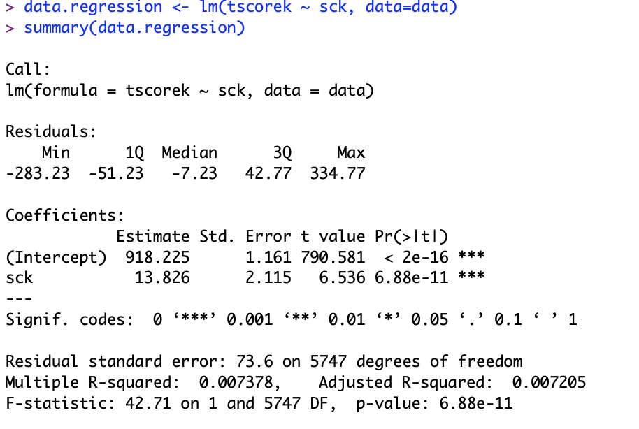
It shows that there is a relationship between the school dummy and test score. The intercepts are continuous variables where the mean value is equal to y (tscorek) when all the regressors are equal to 0.

The sck coefficient represents that an average partial effect has an under dependent variable, meaning that it is a dummy variable that will be represented by either a 1 or 0. Overall, this regression suggests that when a student is assigned to a small classroom (sck), the test score increases by 13.825 points.

Query 3

Show that the OLS estimate of the intercept in this regression will be the sample mean of the test score for those who are in the control group and that the coefficient on sck (small class indicator) will be the difference between the sample mean test score for those in treatment and control groups.

mean(df[which(df$sck==’0′), 3])

mean(df[which(df$sck==’1′), 3])

932.0508 – 918.2251

In the context of regression analysis, it can be demonstrated that the Ordinary Least Squares (OLS) estimate of the intercept in a particular regression is equivalent to the sample mean of the test scores for individuals within the control group. Furthermore, the coefficient associated with the small class indicator (sck) is represented by the disparity between the sample mean test scores for those in the treatment group and those in the control group. Confirming this, the calculated difference between these two means is 13.8257, computed as 932.0508 minus 918.2251.

Query 4

What does this regression say about the impact of class size reductions on students’ performance? Estimate the regression, but now use robust standard errors. Why does the coefficient remain the same? Why does the standard error change?

data.regression <- lmrob(tscorek ~ sck, data=data)

summary(data.regression)

The regression analysis delves into the impact of class size reductions on students’ performance, specifically exploring the relationship between test scores (tscorek) and a small class indicator (sck). Initially, the regression is conducted without robust standard errors, assuming homoskedastic errors. This conventional approach provides an estimate of the coefficient, which, in this case, suggests that when students are moved to a small classroom, their score increases by 13.592.

Subsequently, the regression is re-estimated, this time using robust standard errors. Despite the shift to robust standard errors, the coefficient remains unchanged. The robust standard errors, employed to counteract potential bias introduced by heteroskedastic errors, do not alter the point estimate. However, the standard error undergoes a change. This adjustment is rooted in the nature of robust standard errors, which account for heteroskedasticity and ensure more reliable standard error estimates in the presence of varying error variances.

This validity of using robust standard errors is supported by the fact that most statistical packages allow for their calculation during regression estimation. The heteroskedasticity-robust standard errors, computed through formulas like:

Avar(βˆ|x) = E((x′x)−1(x′uu′x)(x′x)−¹|x)

enable the computation of heteroskedasticity-robust t-statistics and F-statistics. Thus, robust standard errors offer a robust analytical tool in the assessment of regression coefficients and their associated uncertainties.

Question 2

Query 1

Estimate the following regression model:

score = α₀ + α₁sck + α₂Boy + α₃freelunk + α₄totexpk + u (1)

Then run the following regression:

score = β₀ + β₁sck + β₂Boy + β₃freelunk + β₄totexpk + β₅schidkn + v (2)

where schidkn is school identification dummy variables.

data.regression <- lmrob(tscorek ~ sck+boy+freelunk+totexp, data=data)

summary(data.regression)

This output shows that Girls outperform boys by a margin of 13.80328 points in the scores. As totexp is not a binary variable; with each additional year of teaching experience, the student’s score is expected to rise by 1.18.

data.regression <- lmrob(tscorek ~ sck+boy+freelunk+totexp+schidkn, data=data)

summary(data.regression)

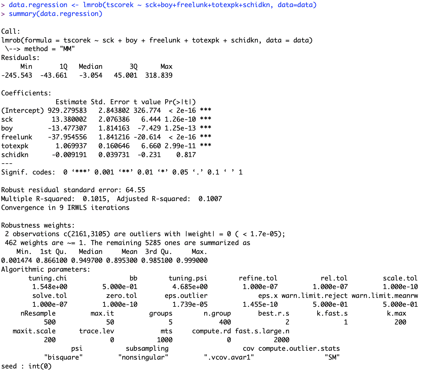
Depending on where the person went to school appears to produce random numbers, so not likely to have an effect on the outcome.

Query 2

Generate a set of dummies for the school ID (schidkn), put it in the other covariates and run the regression again.

mydata <- within(mydata, idnum <- as.numeric(as.factor(schidkn)))

Given we can now identify and capture the effect of belonging to any school, we can more accurately correlate the effect on the score.

mydata <- mydata %>% mutate(idnum = as.factor(schidkn))

model <- lm(tscorek ~ sck + boy + freelunk + totexpk + idnum, data = mydata)

summary(model)

Schools exhibiting positive coefficients indicate higher student performance, whereas those with negative coefficients suggest lower student performance. This valuable insight can now be incorporated into the research findings.

Query 3

What would you expect to happen to the estimate of the treatment effect for small class (β₁) in equation (2) compared to α₁ in equation (1)? Is this what happens?

data.regression <- lmrob(tscorek ~ sck+boy+freelunk+totexp, data=data)

summary(data.regression)

data.regression <- model

summary(data.regression)

When comparing the coefficients of equations 1 and 2, the difference, transitioning from 13.3684 to 15.1331, is not statistically significant. The inclusion of additional variables implies an augmentation of information, thereby enhancing the quality of the information obtained. Consequently, the observed effect is larger than initially anticipated.

Query 4

Consider the following equation:

sck = δ₀ + x₁δ + ε₁ (3)

where x₁=(Boy; freelunk; totexpk).

Now consider a hypothesis test:

δ = (δ₁; δ₂; δ₃)=0.

Does F-test reject the null of δ₁ = δ₂ = δ₃ = 0? What does this test imply for the estimation of α1?

data.regression <- lm(sck ~ boy+freelunk+totexpk, data=data)

summary(data.regression)

Having just conducted an F-Test on the regression model, two key implications emerge:

1. In the context of the research itself, the random assignment to control and treatment groups suggests that factors such as gender, freelunch, and teacher experience should not exert a significant influence on class size. Hence, the coefficients associated with these variables, except for experience, are deemed insignificant. To validate this, a joint test is employed. Additionally, the experiment sheds light on the tendency for teachers with greater experience to be assigned to larger or regular-sized classes.

model <- lm(sck ~ boy + freelunk + totexpk, data = mydata)

test_result <- linearHypothesis(model, c(“boy”, “freelunk”, “totexpk”))

print(test_result)

2. Considering the potential bias in coefficients, including the aforementioned variables as regressors raises the requirement for exogeneity. The variables should remain independent and not interact with each other. If one variable can significantly explain another, particularly in the case of sck, it indicates endogeneity, thereby violating the assumed exogeneity.

In summary, the implications underscore the importance of random assignment in the research design, emphasising the insignificance of certain coefficients and raising concerns about the violation of assumptions, particularly in the case of sck.

Query 5

Consider the following equation:

sck = δ0 + x2γ + ε2 (4)

where x₂=(Boy; freelunk; totexpk; schidkn)

Now consider a hypothesis test of γ=0. Does F-test reject the null of γ₁ = γ₂ = … = γ_p = 0. Is assignment to a small class random?

After examining the p-values, although we will conduct the F-test  for efficiency, direct attention to the joint significance test displayed in the upper section of the table. The rejection is substantial, standing at 0.0000. Despite efforts to control for effects, the reliability of the trials appears questionable. The evidence strongly suggests a pattern where less experienced teachers are more inclined to be assigned to smaller classrooms, while their more experienced counterparts are less likely to be allocated to such settings.

Question 3

Query 1

Generate the interaction of the treatment dummy variable with boy, freelunk and totexpk. What is the mean, standard deviation, minimum and maximum values for each interaction term?

I will make the following interaction terms:

sck*boy: 1 if student is boy AND is assigned to small class, 0 otherwise.

sck*totexpk: total experience of teachers assigned to small classes.

sck*freelunk: 1 if student is receiving free lunch AND is assigned to small class, 0 otherwise.

mydata <- mydata %>%

  mutate(sml_boy = sck * boy,

         sml_freelunch = sck * freelunk,

         sml_exper = sck * totexpk)

Then apply them to the following model:

score = b₀ + b₁sck + b₂boy + b₃freelunk + b₄totexp + b₅boy*sck + b₆freelunk*sck + b₇boy*totexp + u

vars_of_interest <- c(“sml_boy”, “sml_freelunch”, “sml_exper”)

selected_vars <- mydata[, vars_of_interest]

summary_stats <- selected_vars %>%

  summarise_all(list(mean = mean, sd = sd, min = min, max = max))

Note that “sml_exper” ranges from 0 to 27, representing teachers’ experience from the first year to 27 years. The population consists of 15.5% boys and 14.26% individuals receiving free lunch. On average, teachers assigned to small classrooms have 2.7 years of experience.

Regarding these newly created dummy variables, when, for instance, considering the “sml_boy” dummy, it signifies the condition where a student is both a boy and assigned to a small class. The resulting value is a percentage representing the rows meeting this condition with a value of 1. Similar interpretations apply to the other variables. Consequently, it is evident that the earlier mentioned interpretation is expressed as a percentage.

Query 2

Estimate the regression excluding the school dummies but including these interactions. Interpret the coefficients.

model <- lmrob(tscorek ~ sck + boy + freelunk + totexpk + sml_boy + sml_freelunch + sml_exper, data = mydata)

summary(model)

In the regression analysis, school dummies have been excluded, and interactions have been incorporated. On average, boys exhibit a slightly lower performance, with scores 16% less than their counterparts. Students receiving free lunch demonstrate a decrease in performance, with scores 39.49% lower. Each additional year of teaching experience contributes, on average, an increase of 1.66 marks to students’ scores. Boys in the treatment group, assigned to small classes, score 9.73 points more than boys in regular-sized classes. Students with free lunch in the treatment group, assigned to small classrooms, score 0.2779 points less than those in regular-sized classes. In the treatment group with less experienced teachers, students perform 1.63 marks worse on average than those with more experienced teachers.

Query 3

Use an F-test to test the hypothesis that there is the same treatment effect for everyone. Do you accept or reject the test of homogeneity?

test_result <- linearHypothesis(model, c(“sml_boy”, “sml_freelunch”, “sml_exper”))

print(test_result)

Employing an F-test to assess whether the treatment effect is consistent for all subgroups, we examine the hypothesis that the impact of being assigned to a small class is equivalent across boys, students receiving free lunch, and varying levels of teaching experience.

test sml_boy sml_freelunch sml_exper

Upon conducting the test of homogeneity, we find evidence to reject the hypothesis. This rejection implies that the effect of being assigned to a small class differs among subgroups—specifically, boys, students receiving free lunch, and teachers with different levels of experience. Consequently, the conclusion is that classrooms are not homogeneous in terms of the impact of small class assignments. This finding contradicts the assumption of uniform treatment effects and underscores the importance of considering subgroup variations in the assessment of the impact of class size on different demographic and experiential categories.