Homework from 2 weeks ago

This is how mine looks:

Sharpe Ratio:

=IFERROR((P4–$P$2)/VLOOKUP(A4,Stocks!$A$1:$AI$1,COUNTA($A$4:A4)*7–5,1))

First, I created a new sheet called ‘Stocks’ then selected the ticker for each one:

Then I used the following formula to capture the data from this website – https://www.marketwatch.com :

=ARRAYFORMULA(SUBSTITUTE(IMPORTHTML(“https://www.marketwatch.com/investing/stock/”&A1&“/download-data?countrycode=au&mod=mw_quote_tab”,“table”,5),“$”,))

Some of the websites needed slight adjustments, i.e.:

=ARRAYFORMULA(SUBSTITUTE(IMPORTHTML(“https://www.marketwatch.com/investing/stock/”&H1&“/download-data?mod=mw_quote_tab”,“table”,5),“$”,))

Then I created a column of numbered Close values, as they imported as text:

=VALUE(E3)

From here, I was able to each stock’s standard deviation:

=STDEV(G3:G20)

Going back to the Dashboard, I had to construct this formula:

=IFERROR((P4–$P$2)/VLOOKUP(A4,Stocks!$A$1:$AI$1,COUNTA($A$4:A4)*7–5,1))

The VLOOKUP function is accounting for the number of columns between each of the stock’s standard deviation so that I didn’t have to manually account for each one.

Lastly, I used a fuzzy-match VLOOKUP formula to report the type of ratio it was:

Do you understand my caveat now from last week – this is NOT financial advice. Moving on…

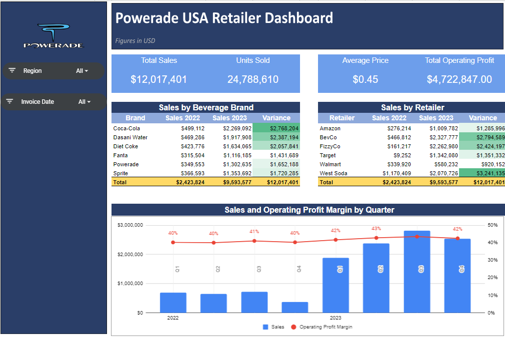
Sales Dashboard

https://docs.google.com/spreadsheets/d/1Y41xUwBQgN5hC5DQd0m7GE60OsfJsghTBZA2YZfxRNw/edit#gid=1699220080