This is a brief message to say happy holidays, if you are in fact celebrating it.

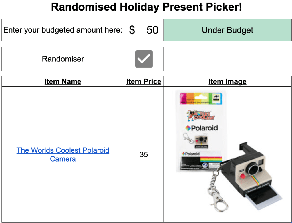
What would this post be without a Google Spreadsheet activity, so here it is; the Randomised Holiday Present Picker! Need a (very) last minute holiday present idea? Use this randomiser to generate some ideas.

https://docs.google.com/spreadsheets/d/1wWKxHtIS1ojlObI6T_3bXMfFoM2QbA1nb9zOajFEpDw/edit?gid=0#gid=0

Here’s a brief breakdown of the formulas that can be found in the ‘Inventory’ sheet:

Inventory Sheet

Item Number

=SEQUENCE(COUNTA(B2:B))

Automatically counting the number of items that appear in the IMPORTXML function (see next).

Item Name

=ARRAYFORMULA(SUBSTITUTE(SUBSTITUTE(INDEX(IMPORTXML(“https://www.ebay.com.au/str/hecticgifts”, “//*[@id=’mainContent’]/div/div[1]/div[2]/section[7]/section//h3”),,2),“NEW “,),“- “,))

Found a webpage with numerous items to draw upon. I first imported the data then wanted to isolate the titles, so I wrapped the INDEX function around the IMPORTXML. The following two SUBSTITUTE functions were added to clean the data of their “NEW” and “- “ qualitative marketing tactics. Although there will be some information added in the prefix of the present titles, this doesn’t distract too much from the overall idea.

Item Price

This one was actually the trickiest portion to obtain. I originally started with this code, but I was receiving F#0 in lieu of prices and this was offsetting the output, which would throw off my lookup values:

I started coding out an elongated formula, but then I remembered about the LET function. Here is my final function; I’ll break it down for you:

=LET(

rawData, INDEX(IMPORTXML(“https://www.ebay.com.au/str/hecticgifts”, “//*[@id=’mainContent’]/div/div[1]/div[2]/section[7]/section//article/div[3]/div/div/span”), , 1),

 filteredData, ARRAYFORMULA(IF(rawData = “F#0”, NA(), rawData)),

nonEmptyData, FILTER(filteredData, NOT(ISNA(filteredData))),

cleanedData, ARRAYFORMULA(RIGHT(nonEmptyData, LEN(nonEmptyData) – 4)),

cleanedData)

I assigned my original INDEX web page lookup as the rawData variable:

rawData, INDEX(IMPORTXML(“https://www.ebay.com.au/str/hecticgifts”, “//*[@id=’mainContent’]/div/div[1]/div[2]/section[7]/section//article/div[3]/div/div/span”), , 1)

Then I filtered the DATA, using the IF function to replace the F#0 outputs with an NA() output. If this wasn’t an error, then it would print the next element in the rawData output:

 filteredData, ARRAYFORMULA(IF(rawData = “F#0”, NA(), rawData))

Next was to filter out these NA() functions that were outputting in the filteredData variable:

nonEmptyData, FILTER(filteredData, NOT(ISNA(filteredData)))

With that completed, it meant that I had to finally standardise the value output by removing the first 4 characters of the price output:

cleanedData, ARRAYFORMULA(RIGHT(nonEmptyData, LEN(nonEmptyData) – 4)),

Item Image

Going back to a previous blog post regarding my data analyst road map (and my weather dashboard) where I used this same process, I used the IMAGE function to display the present image in the cell — something that I can use for the lookup function on the first page:

=ARRAYFORMULA(IMAGE(IMPORTXML(“https://www.ebay.com.au/str/hecticgifts”, “//*[@id=’mainContent’]/div/div[1]/div[2]/section[7]/section//img/@src”)))

Picker Sheet

With all of that information sorted, I then created the randomiser on the first page. I used 3 different variations on a simple VLOOKUP function. Overall, here was my process.

Randomiser

Create a randomised number generator that is dependent on the number of items that are inputted by ‘Item Number’ on the Inventory sheet:

=RANDBETWEEN(Inventory!A2,Inventory!A49)

Item Name

Item Name VLOOKUP

=HYPERLINK(“https://www.ebay.com.au/str/hecticgifts”,VLOOKUP($E$9,Inventory!$A$2:$D,COLUMN(B8),0))

I wanted people to be able to click on the item to peruse it, should they wish. So, I wrapped the VLOOKUP function (random_itemNumber_geneator, Inventorydataset,currentColumnForEaseOfDraggingTheFormulaAcross,exactMatch) in a HYPERLINK function, allowing people to be directed to the website.

Item Price

Item Price VLOOKUP

=VALUE(VLOOKUP($E$9,Inventory!$A$2:$D,COLUMN(C8),0))

This data was being pulled from the Inventory sheet, which was being pulled (as text) from the IMPORTXML process. Like the Item Name VLOOKUP, I imposed a similar approach for the VLOOKUP process, but wrapped in a VALUE function, given that all of the redundant information/formatting has already been stripped. This means that I can compare this value for the user’s budget (see below).

Item Image

Item Image VLOOKUP

=VLOOKUP($E$9,Inventory!$A$2:$D,COLUMN(D8),0)

I have already gone to the trouble of pulling the image source from the IMPORTXML process, so this was legitimately just looking up the correct image.

Randomiser

This is just a checkbox (Menu: Insert > Checkbox) that people can press to trigger the randomiser on the sheet. Simply pressing delete/backspace on an empty cell has the same processing effect.

Budget checker

Given that this could be used for a Secret Santa type scenario, I thought it was a good idea to integrate a budget checker. Ideally, you’d filter the results by their budget, but that is a potential future improvement. This is a standard IF function that checks the present value against the budget and provides conditional formatting for the user:

=IF(C8>C3,“Over Budget! Pick Again.”,“Under Budget”)

Well, that’s it! Have a safe and happy holiday. I hope that you enjoyed this post!